# Libraries
library(ggplot2)
library(dplyr)
library(ggrepel)
library(DT)
library(qqman)
library(knitr)

In addition to the classical GWA analyses, we ran a variance QTL (vQTL) GWA analysis. Wang et al. 2019 have recently shown that gene-by-environment (GxE) interactions can be inferred from vQTLs. Here, used OSCA to identify vQTLs for vitamin D levels.

Below we describe our analysis and present the results.

Methods

Data

The following files were used to run the analysis:

Phenotype file:This file includes one line per individual and a column with the phenotype. The phenotype was obtained after regressing out the effect of confouders, removing outliers and standardising the residuals. For more information on how the phenotype was generated and what covariates were used see the Prepare phenotype section in the Pheno tab. In total 318851 unrelated individuals of European ancestry were analysed.
Genotype file: This analysis was restricted to unrelated individuals of European ancestry and included 44741804 autossomal variants with (1) minor allele count (MAC) > 5, (2) info score (INFO) > 0.3, and (3) genotype missingness > 0.05. In addition, we excluded variants with missingness < 0.05, pHWE < 1x10^-5, and MAC > 5 in the subset of unrelated European individuals.

GWAS

This analysis was performed using the Levene’s median test implemented in OSCA. We restricted the analysis to SNPs with MAF>0.05 to avoid spurious associations due to coincidence of low-frequency variants with phenotype outliers (see Wang et al. 2019 for more information).

# Make list of SNPs to keep in the analysis, excluding duplicated SNPs
geno=$medici/v3EURu_impQC/ukbEURu_imp_chr{TASK_ID}_v3_impQC
filters=maf0.01
genoDir=$WD/input/UKB_v3EURu_impQC
snpList=$genoDir/UKB_impQC_noDuplicated_$filters
cd $genoDir
tmp_command="plink --bfile $geno \
                   --exclude $WD/input/UKB_v3EUR_impQC/UKB_EUR_impQC_duplicated_rsIDs \
                   --maf 0.01 \
                   --make-bed \
                   --out ${snpList}_chr{TASK_ID}"
qsubshcom "$tmp_command" 1 5G makeBED.`basename $snpList` 3:00:00 "-array=1-22"
cat ${snpList}_chr*.snplist > $snpList.snplist
rm ${snpList}_chr*

# Make list of variants with MAF>0.05 - we will restrict results to this set (see below)
geno=$medici/v3EURu_impQC/ukbEURu_imp_chr{TASK_ID}_v3_impQC
filters=maf0.05
genoDir=$WD/input/UKB_v3EURu_impQC
snpList=$genoDir/UKB_impQC_$filters
cd $genoDir
tmp_command="plink --bfile $geno \
                   --maf 0.05 \
                   --write-snplist \
                   --out ${snpList}_chr{TASK_ID}"
qsubshcom "$tmp_command" 1 5G `basename $snpList` 3:00:00 "-array=1-22"
cat ${snpList}_chr*.snplist > $snpList.snplist
rm ${snpList}_chr*


# #########################################
# Run vQTL GWAS with OSCA
# #########################################

# Set directories
results=$WD/results/vqtl
tmpDir=$results/tmpDir

# Files/settings to use
prefix=vitD_vqtlGWAS
geno=$WD/input/UKB_v3EURu_impQC/UKB_impQC_noDuplicated_maf0.01_chr{TASK_ID}
pheno=$WD/input/vqtl_pheno
output=$tmpDir/${prefix}_chr{TASK_ID}
snps2include=$WD/input/UKB_v3EURu_impQC/UKB_impQC_noDuplicated_maf0.01.snplist

# Run GWAS
cd $results
osca=$bin/osca/osca_v0.45
tmp_command="$osca --bfile $geno \
                   --maf 0.01 \
                   --extract-snp $snps2include\
                   --pheno $pheno \
                   --vqtl \
                   --vqtl-mtd 2 \
                   --out $output"

qsubshcom "$tmp_command" 1 300G $prefix 30:00:00 "-array=1-22"


# Merge results from each chr after all have finished running (both the standard .vqtl output and the new .ma format)
echo "SNP A1 A2 freq b se p n" | tr ' ' '\t'> $results/$prefix.ma
cat $tmpDir/${prefix}_chr*ma | grep -v 'SNP' >> $results/$prefix.ma

sed 1q $tmpDir/${prefix}_chr1.vqtl > $results/$prefix.vqtl
cat $tmpDir/${prefix}_chr*vqtl | grep -v 'SNP' >> $results/$prefix.vqtl
gzip $results/$prefix.vqtl



# Check if there is an inflation of assoications among rare (MAF<0.05) variants
# qsub -I -A UQ-IMB-CNSG -X -l nodes=1:ppn=5,mem=20GB,walltime=6:00:00
#  cd $WD
# R
# freq=read.table("input/UKB_v3EURu_impQC/v3EURu.frq",h=T,stringsAsFactors=F)
 #osca=read.table("results/vqtl/vitD_vqtlGWAS.ma",h=T,stringsAsFactors=F)
 #df=merge(osca,freq[,c("SNP","MAF")])
 #df=df[df$p<5e-8,]
 #plot(df$p~df$MAF)
 #abline(v=0.05)
 #nrow(df[df$MAF<.05,]) ## 460
 #nrow(df[df$MAF>=.05 & df$MAF<.1,]) ## 666
 #There may be some inflation. We may be better restricting to variants with MAF>0.05 as Wang et al. 2019 did.

# Restrict results to variants with MAF>0.05
filters=maf0.05
sed 1q $results/$prefix.ma > $results/$prefix.$filters.ma
awk 'NR==FNR{a[$1];next} ($1 in a)' $WD/input/UKB_v3EURu_impQC/UKB_impQC_$filters.snplist $results/$prefix.ma >> $results/$prefix.$filters.ma

zcat $results/$prefix.vqtl.gz | sed 1q > $results/$prefix.$filters.vqtl
awk 'NR==FNR{a[$1];next} ($2 in a)' $WD/input/UKB_v3EURu_impQC/UKB_impQC_$filters.snplist <(zcat $results/$prefix.vqtl.gz) >> $results/$prefix.$filters.vqtl
gzip $results/$prefix.$filters.vqtl

Clump

Results were then clumped with plink 1.9, using the following options:

–clump-p1 = 5x10^-8 - max P-value for index variants to start a clump
–clump-p2 = 0.01 (default) - max P-value for variants in a clump to be listed in column SP2
–clump-r2 = 0.01 - minimum r2 with index variant for a site to be included in that clump
–clump-kb = 5000 - maximum distance from index SNP for a site to be included in that clump

# #########################################
# Clump GWAS results
# #########################################

# Directories
results=$WD/results/vqtl
tmpDir=$results/tmpDir

# Files/settings to use
prefix=vitD_vqtlGWAS
ref=$medici/v3EURu_impQC/ukbEURu_imp_chr{TASK_ID}_v3_impQC
inFile=$tmpDir/${prefix}_chr{TASK_ID}.vqtl
outFile=$tmpDir/${prefix}_chr{TASK_ID}
snps2exclude=$WD/input/UKB_v3EUR_impQC/UKB_EUR_impQC_duplicated_rsIDs
snps2include=$WD/input/UKB_v3EURu_impQC/UKB_impQC_maf0.05.snplist

# Run clumping
cd $results
plink=$bin/plink/plink-1.9/plink
tmp_command="$plink --bfile $ref \
                    --extract $snps2include \
                    --exclude $snps2exclude \
                    --clump $inFile \
                    --clump-p1 5e-8 \
                    --clump-r2 0.01 \
                    --clump-kb 5000 \
                    --clump-field "P" \
                    --out $outFile"          
qsubshcom "$tmp_command" 1 30G $prefix.clump 24:00:00 "-array=1-22"


# Merge clumped results once all chr finished running
cat $tmpDir/${prefix}_chr*clumped | grep "CHR" | head -1 > $results/$prefix.maf0.05.clumped
cat $tmpDir/${prefix}_chr*clumped | grep -v "CHR" |sed '/^$/d'  >> $results/$prefix.maf0.05.clumped

LDSC

To run LDSC, we restricted the GWAS summary statistics to variants found in w_hm3.noMHC.snplist (downloaded from LDHub). This is a list of HapMap3 SNPs that excludes variants in the MHC region.

module load ldsc
prefix=vitD_vqtlGWAS

# Directories
results=$WD/results/vqtl
tmpDir=$results/tmpDir
ldscDir=$bin/ldsc

# Format GWAS results
awk '{print $1,$2,$3,$5,$8,$7}' $results/$prefix.maf0.05.ma > $tmpDir/$prefix.ldHubFormat

# Restrict to common SNPs
sed 1q $tmpDir/$prefix.ldHubFormat > $results/$prefix.ldHubFormat
awk 'NR==FNR{a[$1];next} ($1 in a)' $WD/input/UKB_v3EURu_impQC/UKB_EURu_impQC_maf0.01.snplist <(awk 'NR==FNR{a[$1];next} ($1 in a)' $WD/input/w_hm3.noMHC.snplist $tmpDir/$prefix.ldHubFormat) >> $results/$prefix.ldHubFormat

# Munge sumstats (process sumstats and restrict to HapMap3 SNPs)
munge_sumstats.py --sumstats $results/$prefix.ldHubFormat \
                  --merge-alleles $ldscDir/w_hm3.snplist \
                  --out $tmpDir/$prefix
                  
# Run LDSC
ldsc.py --h2 $tmpDir/$prefix.sumstats.gz \
        --ref-ld-chr $ldscDir/eur_w_ld_chr/ \
        --w-ld-chr $ldscDir/eur_w_ld_chr/ \
        --out $results/$prefix.ldsc

GxE

To assess whether the vQTLs identified reflect gene-environment (GxE) interactions with season of blood draw we performed a GxE analysis with plink 1.9, using the following options:

bfile: We restricted the analysis to unrelated individuals of European ancestry and included 44741804 autossomal variants with (1) minor allele count (MAC) > 5, (2) info score (INFO) > 0.3, and (3) genotype missingness > 0.05. In addition, we excluded variants with missingness < 0.05, pHWE < 1x10^-5, and MAC > 5 in the subset of unrelated European individuals.
allow-no-sex
linear
pheno: Briefly, the phenotype was pre-adjusted for age, assessment centre, assessment month, genotyping batch and 40 PCs within different groups of sex and vitamin supplement intake and residuals were normalised with a rank-based inverse-normal transformation. See the Prepare phenotype section in Pheno for more detail.
gxe: We used this option, together with --covar, to test whether the association with vitamin D differed in two seasons (see more details of how season was defined in Pheno > Prepare phenotype > Season-stratified GWAS).

# Set directories
results=$WD/results/gxe
tmpDir=$results/tmpDir

# Files/settings to use
prefix=vitD_season_gxe
geno=$medici/v3EURu_impQC/ukbEURu_imp_chr{TASK_ID}_v3_impQC
pheno=$WD/input/plink_pheno
season=$WD/input/covariates_season
output=$tmpDir/${prefix}_chr{TASK_ID}
snps2include=$WD/input/UKB_v3EURu_impQC/UKB_impQC_noDuplicated_maf0.01.snplist

# Generate file with season only
seasonCovar=$tmpDir/season
awk '{print $1,$2,$5}' $season > $seasonCovar

# Run analysis
cd $results
plink=$bin/plink/plink-1.9/plink
tmp_command="$plink --bfile $geno \
                    --extract $snps2include \
                    --allow-no-sex \
                    --linear \
                    --pheno $pheno \
                    --pheno-name norm_vitD_res \
                    --gxe \
                    --covar $seasonCovar \
                    --out $output"
qsubshcom "$tmp_command" 1 30G gxe 24:00:00 "-array=1-22"

# Merge results from each chr after all have finished running
sed 1q $tmpDir/${prefix}_chr1.qassoc.gxe | awk -v OFS="\t" '$1=$1'  > $results/$prefix.qassoc.gxe
cat $tmpDir/${prefix}_chr*.qassoc.gxe | grep -v 'CHR' | awk -v OFS="\t" '$1=$1' >> $results/${prefix}.qassoc.gxe
gzip $results/$prefix.qassoc.gxe

# Restrict results to variants with MAF>0.05
filters=maf0.05
zcat $results/$prefix.qassoc.gxe.gz | sed 1q > $results/$prefix.$filters.qassoc.gxe
awk 'NR==FNR{a[$1];next} ($2 in a)' $WD/input/UKB_v3EURu_impQC/UKB_impQC_$filters.snplist <(zcat $results/$prefix.qassoc.gxe.gz) >> $results/$prefix.$filters.qassoc.gxe
gzip $results/$prefix.$filters.qassoc.gxe

After restricting the GxE results to variants with MAF > 0.05 (same as used in vQTL analysis) results were clumped with plink 1.9, using the following options:

–bfile - samples from unrelated EUR were used as reference
–clump-p1 = 5x10^-8 - max P-value for index variants to start a clump
–clump-p2 = 0.01 (default) - max P-value for variants in a clump to be listed in column SP2
–clump-r2 = 0.01 - minimum r2 with index variant for a site to be included in that clump
–clump-kb = 5,000 - maximum distance from index SNP for a site to be included in that clump

# #########################################
# Clump GxE results
# #########################################

# Directories
results=$WD/results/gxe
tmpDir=$results/tmpDir

# Files/settings to use
prefix=vitD_season_gxe.maf0.05
ref=$medici/v3EURu_impQC/ukbEURu_imp_chr{TASK_ID}_v3_impQC
inFile=$results/$prefix.qassoc.gxe.gz
outFile=$tmpDir/${prefix}_chr{TASK_ID}
snps2exclude=$WD/input/UKB_v3EUR_impQC/UKB_EUR_impQC_duplicated_rsIDs

# Run clumping
cd $results
plink=$bin/plink/plink-1.9/plink
tmp_command="$plink --bfile $ref \
                    --exclude $snps2exclude \
                    --clump $inFile \
                    --clump-p1 5e-8 \
                    --clump-r2 0.01 \
                    --clump-kb 5000 \
                    --clump-field "P_GXE" \
                    --out $outFile"          
qsubshcom "$tmp_command" 1 30G $prefix.clump 24:00:00 "-array=1-22"

# #########################################
# Merge clumped results once all chr finished running
# #########################################
cat $tmpDir/${prefix}_chr*clumped | grep "CHR" | head -1 > $results/${prefix}.clumped
cat $tmpDir/${prefix}_chr*clumped | grep -v "CHR" |sed '/^$/d'  >> $results/${prefix}.clumped

Results

vQTL Manhattan plot

# Read in vQTL GWAS results ----------------------------------------
#gwas=read.table("results/vqtl/vitD_vqtlGWAS.maf0.05.vqtl.gz", h=T, stringsAsFactors=F)
#saveRDS(gwas, file="results/vqtl/vitD_vqtlGWAS.vqtl.RDS")
gwas=readRDS("results/vqtl/vitD_vqtlGWAS.vqtl.RDS")
names(gwas)[grep("Chr|bp|beta",names(gwas))]=c("CHR","BP","BETA")
clump=read.table("results/vqtl/vitD_vqtlGWAS.maf0.05.clumped", h=T, stringsAsFactors=F)

# Add cumulative position + clumping/cojo information for plotting
  # ----- Add chromosome start site to the GWAS result
  don=aggregate(BP~CHR,gwas,max)
  don$tot=cumsum(as.numeric(don$BP))-don$BP
  don=merge(gwas,don[,c("CHR","tot")])
  # ----- Add a cumulative position to plot in this order
  don=don[order(don$CHR,don$BP),]
  # ----- Restrict SNPs with P<0.03 + a random samples of 100K SNPs (to plot faster)
  don=don[don$P<0.03 | don$SNP %in% sample(gwas$SNP,100000),]
  don$BPcum=don$BP+don$tot
  # ----- Add clump information
  don$is_clump_lead=ifelse(don$SNP %in% clump$SNP, "yes","no")

  # ----- Prepare X axis
  options(warn=-1)  
  axisdf = don %>% group_by(CHR) %>%  summarise(center=( max(BPcum) + min(BPcum) ) / 2 )
  options(warn=0)
  
# Generate Manhattan plot
ggplot(don, aes(x=BPcum, y=-log10(P))) +
  geom_point( aes(color=as.factor(CHR)), alpha=0.3, size=0.5) +
  scale_color_manual(values = rep(c("lightsteelblue4", "lightsteelblue3"),44)) +
  # Highlighted SNPs of interest
  geom_point(data=don[don$is_clump_lead=="yes",], color="red", size=2) +
  geom_label_repel( data=don[don$is_clump_lead=="yes",], aes(label=SNP), size=2) +
  # Make X axis
  scale_x_continuous( label=axisdf$CHR, breaks=axisdf$center ) +
  labs(x="")+
  theme_bw() +
  theme(legend.position="none",
        panel.border = element_blank(),
        panel.grid.major.x = element_blank(),
        panel.grid.minor.x = element_blank())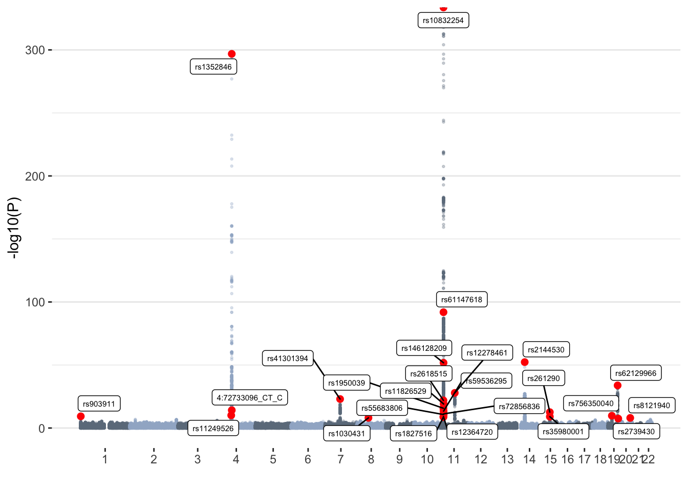

# Keep info to summarise in the report below
oscaGWAS_common=gwas
oscaGWAS_clump_common=clump
vqtl_snps=clump$SNP

Red dots represent lead SNPs in independent loci identified with Clump.

Summary of vQTL results

Briefly, we have:

6098063 variants tested
4008 GWS (P<5x10^-8) associations (vQTLs)
25 independent loci (determined through clumping)

# fastGWA results
#gwas=read.table("results/fastGWA/vitD_fastGWA_withX.gz", h=T, stringsAsFactors=F)
#saveRDS(gwas, file="results/fastGWA/vitD_fastGWA_withX.RDS")
fastGWA_common=readRDS("results/fastGWA/vitD_fastGWA_withX.RDS")
names(fastGWA_common)[grep("POS",names(fastGWA_common))]=c("BP")
fastGWA_cojo_common=read.table("results/fastGWA/vitD_fastGWA_maf0.01_withX.cojo", h=T, stringsAsFactors=F)

# vQTLs and QTLs
qtls=fastGWA_common[fastGWA_common$P<5e-8,"SNP"]
vqtls=oscaGWAS_common[oscaGWAS_common$P<5e-8,"SNP"]
clumped_vqtls=oscaGWAS_clump_common$SNP

vqtls_tested_in_GWAS=nrow(fastGWA_common[fastGWA_common$SNP %in% oscaGWAS_clump_common$SNP,])

Comparing with results from the fastGWA analysis:

3454 of the 4008 vQTLs were also QTLs, i.e. passed the genome-wide (P<5x10^-8) significance threshold in the QTL analysis (fastGWA)
Of the 25 lead vQTLs in independent loci, 25 were tested in the QTL analysis (fast-GWA), and:
- 23 were also QTLs
- 2 were exclusively vQTLs

indep = oscaGWAS_common[oscaGWAS_common$SNP %in% oscaGWAS_clump_common$SNP,]
names(indep)[grep("se",names(indep))]="SE"

# Add statitics from main GWAS (QTL)
  indep=merge(indep, fastGWA_common[,c("SNP","BETA","SE","P")], by="SNP", suffixes=c("","_QTL"))

# Add statistics from stratified GWAS
  #summer=read.table("results/stratifiedGWAS/vitD_summerGWAS.gz", h=T, stringsAsFactors=F)
  #saveRDS(summer, file="results/stratifiedGWAS/vitD_summerGWAS.RDS")
  summer=readRDS("results/stratifiedGWAS/vitD_summerGWAS.RDS")
  #winter=read.table("results/stratifiedGWAS/vitD_winterGWAS.gz", h=T, stringsAsFactors=F)
  #saveRDS(winter, file="results/stratifiedGWAS/vitD_winterGWAS.RDS")
  winter=readRDS("results/stratifiedGWAS/vitD_winterGWAS.RDS")
  
  indep=merge(indep, summer[,c("SNP","BETA","SE","P")], by="SNP", suffixes=c("","_summer"))
  indep=merge(indep, winter[,c("SNP","BETA","SE","P")], by="SNP", suffixes=c("","_winter"))

# Add statistics from GxE analyses with season
  ## GxE with PLINK
  gxe=read.table("results/gxe/vitD_season_gxe.qassoc.gxe.gz", h=T, stringsAsFactors=F)
  indep=merge(indep, gxe[,c("SNP","Z_GXE","P_GXE")])

# Identify vQTL types in list of independet associations
indep$type=ifelse(indep$SNP %in% qtls, "vQTL + QTL", "vQTL")

# Format table
indep=indep[,c("type","SNP","CHR","BP","A1","A2","freq","NMISS","BETA","SE","P","BETA_QTL","SE_QTL","P_QTL","BETA_summer","SE_summer","P_summer","BETA_winter","SE_winter","P_winter","Z_GXE","P_GXE")]
  ## Round P-values
  cols=c("P","P_QTL","P_summer","P_winter","P_GXE")
  indep[,cols]=apply(indep[,cols], 2, function(x){format(x, digits=3)})
  ## Round betas and SE
  cols=c("SE","SE_QTL","SE_summer","SE_winter","BETA","BETA_QTL","BETA_summer","BETA_winter")
  indep[,cols]=apply(indep[,cols], 2, function(x){round(x, 4)})
  ## Round freq
  indep$freq=round(indep$freq, 2)
  ## Convert numeric columns to numeric
  #numericCols=c("CHR","BP","freq","NMISS","BETA","SE","P","BETA_QTL","SE_QTL","P_QTL","BETA_summer","SE_summer","P_summer","BETA_winter","SE_winter","P_winter","Z_GXE","P_GXE")
#indep[,numericCols] = apply(indep[,numericCols], 2, function(x) as.numeric(as.character(x)))
indep=indep[order(as.numeric(indep$P)),]

# Present table
datatable(indep, 
          rownames=FALSE, 
          extensions=c('Buttons','FixedColumns'),
          options=list(pageLength=10,
                       dom='frtipB',
                       buttons=c('csv', 'excel'),
                       scrollX=TRUE),
          caption="List of lead vQTLs in independent loci") %>% 
  formatStyle("type","white-space"="nowrap") %>% 
  formatStyle("P","white-space"="nowrap")

Columns are: type, type of QTL; SNP, SNP rs ID; CHR, chromosome; BP, physical position; A1, A2, effect allele and other allele, respectively; freq, frequency of the effect allele in the original data; NMISS, sample size in vQTL GWAS; BETA, SE and P, effect size, standard error and P-value from the vQTL GWAS; BETA_QTL, SE_QTL and P_QTL, effect size, standard error and P-value from the main QTL GWAS; BETA_summer, SE_summer, P_summer, BETA_winter, SE_winter and P_winter, effect size, standard error and P-values obtained in season-stratified GWAS (includes related EUR); Z_GXE and P_GXE, z-score and P-value from GxE analysis with season (PLINK results).

vQTL QQplot + LDSC

# Get sample for QQ plotting
pthrh=0.03
tmp=c(oscaGWAS_common[oscaGWAS_common$P<pthrh,"P"], sample(oscaGWAS_common[oscaGWAS_common$P>pthrh,"P"],100000))

# Plot
qq(tmp)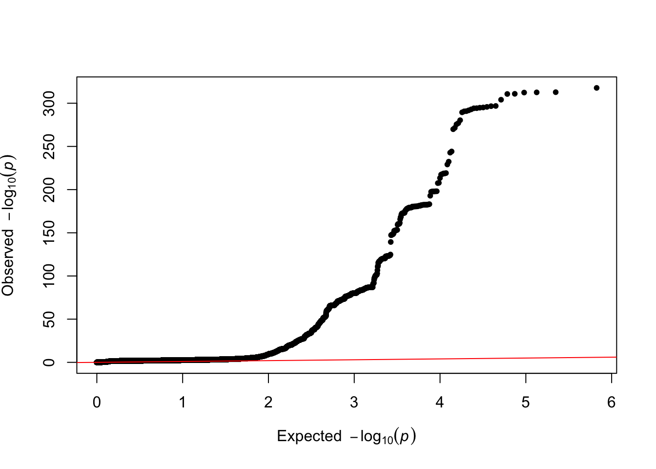

LDSC

tmp=read.table("results/vqtl/vitD_vqtlGWAS.ldsc.log", skip=15, fill=T, h=F, colClasses="character", sep="_")[,1]

# Get results:
h2=strsplit(grep("Total Observed scale h2",tmp, value=T),":")[[1]][2]
lambda_gc=strsplit(grep("Lambda GC",tmp, value=T),":")[[1]][2]
chi2=strsplit(grep("Mean Chi",tmp, value=T),":")[[1]][2]
intercept=strsplit(grep("Intercept",tmp, value=T),":")[[1]][2]
ratio=strsplit(grep("Ratio",tmp, value=T),":")[[1]][2]

Total Observed scale h²: 0.0277 (0.0117)
Lambda GC: 1.0988
Mean Chi²: 1.2059
Intercept: 1.0235 (0.0087)
Ratio: 0.1143 (0.0421)

GxE with season

To assess whether the vQTLs identified reflect gene-environment (GxE) interactions with season of blood draw we performed a GxE analysis with season (Winter=Dec-Apr; Summer=Jun-Oct).

# #############################
# GxE with environment - GWA
# #############################
gxe=read.table("results/gxe/vitD_season_gxe.maf0.05.qassoc.gxe.gz", h=T, stringsAsFactors=F)

# Identify independent GxE results (clump)
clumps=read.table("results/gxe/vitD_season_gxe.maf0.05.clumped", h=T, stringsAsFactors=F)
gxe$indep_GXE=ifelse(gxe$SNP %in% clumps$SNP, "Yes","No")

# Identify independent vQTLs (clump)
gxe$vQTL=ifelse(gxe$SNP %in% oscaGWAS_common[oscaGWAS_common$P<5e-8,"SNP"], "Yes","No")
gxe$indep_vQTL=ifelse(gxe$SNP %in% oscaGWAS_clump_common$SNP, "Yes","No")

# Restrict to GWS GxE
gwsGXE=gxe[gxe$P_GXE<5e-8,]

# Add vQTL sumstats
tmp=oscaGWAS_common[,c("SNP","BETA","se","P")]
names(tmp)=c("SNP","b_vQTL","se_vQTL","P_vQTL")
gwsGXE=merge(gwsGXE, tmp)

# Add stratified GWAS results
winter=readRDS("results/stratifiedGWAS/vitD_winterGWAS.RDS")
summer=readRDS("results/stratifiedGWAS/vitD_summerGWAS.RDS")
names(winter)=paste0(names(winter),"_winter")
names(summer)=paste0(names(summer),"_summer")
gwsGXE=merge(gwsGXE, winter[,paste0(c("SNP","POS","BETA","SE","P"), "_winter")], all.x=T, by.x="SNP", by.y="SNP_winter")
gwsGXE=merge(gwsGXE, summer[,paste0(c("SNP","BETA","SE","P"), "_summer")], all.x=T, by.x="SNP", by.y="SNP_summer")
names(gwsGXE)[grep("POS_winter", names(gwsGXE))]="BP"

We tested 6098063 variants with MAF > 0.05, and found:

1127 GWS GxE associations
- 1120 (99.38%) also GWS in vQTL analysis
- 7 (0.62%) not GWS in vQTL analysis
6096936 GxE associations that were not GWS
- 2888 (0.05%) GWS in vQTL
- 6094048 (99.95%) not GWS in vQTL analysis
5 independent GxE loci
- 4 GWS in vQTL analysis
5 of the 25 independent vQTLs had a GWS interaction with season

# Format table
gwsGXE$P_GXE=format(gwsGXE$P_GXE, digits=3)
gwsGXE$P_winter=format(gwsGXE$P_winter, digits=3)
gwsGXE$P_summer=format(gwsGXE$P_summer, digits=3)
gwsGXE$P_vQTL=format(gwsGXE$P_vQTL, digits=3)
gwsGXE=gwsGXE %>% mutate_at(vars(BETA1, SE1, BETA2, SE2, BETA_summer, SE_summer, BETA_winter, SE_winter, b_vQTL, se_vQTL), round, 4)

# Order columns
gwsGXE=gwsGXE[,c("SNP","CHR","BP","NMISS1","BETA1","SE1","NMISS2","BETA2","SE2","Z_GXE","P_GXE","indep_GXE","indep_vQTL","b_vQTL","se_vQTL","P_vQTL","BETA_winter","SE_winter","P_winter","BETA_summer","SE_summer","P_summer")]

# Present table
datatable(gwsGXE, 
          rownames=FALSE, 
          extensions=c('Buttons','FixedColumns'),
          options=list(pageLength=10,
                       dom='frtipB',
                       buttons=c('csv', 'excel'),
                       scrollX=TRUE),
          caption="GxE results for variants with MAF > 0.05 and P_GXE<5e-8")

Columns are: SNP, SNP rs ID; CHR, Chromosome; BP, base pair;NMISS1, BETA1 and SE1 , Non-missing genotype calls, regression coefficient, and standard error for first group (winter); NMISS2, BETA2 and SE2 , Non-missing genotype calls, regression coefficient, and standard error for first group (summer); Z_GXE and P_GXE, Z score and asymptotic p-value test for interaction term; “indep_GXE”, whether the interaction term was independent by LD; indep_vQTL whether the SNP was a lead SNP in the clumped vQTL results; BETA, SE, and P with suffix _vQTL are from the vQTL GWAS, and those with suffixes _winter and _summer are results from the season-stratified GWA analyses.

# #############################
# GxE with environment - lead vQTLs only - calculated in R
# #############################

df=read.table("results/vqtl/GxEresults", h=T, stringsAsFactors=F)
df$b_raw=round(df$b_raw,4)
df$b_adj=round(df$b_adj,4)
df$p_raw=format(df$p_raw, digits=3)
df$p_adj=format(df$p_adj, digits=3)

# Present table
datatable(df, 
          rownames=FALSE, 
          extensions=c('Buttons','FixedColumns'),
          options=list(pageLength=10,
                       dom='frtipB',
                       buttons=c('csv', 'excel'),
                       scrollX=TRUE),
          caption=paste0("GxE associations between the ",nrow(df)," lead vQTLs and season")) %>% 
  formatStyle("p_raw","white-space"="nowrap")



#Columns are: **vQTL**, SNP rs ID; **b_raw** and **p_raw**, effect size and P-value from GxE analysis with environment - using the raw phenotype (i.e. raw vitamin D levels); **b_adj** and **p_adj**, effect size and P-value from GxE analysis with environment - using the phenotype used in the vQTL GWAS (i.e. pre-adjusted for covariates and standardised after removing outliers).

# Get GxE results for independent vQTLs
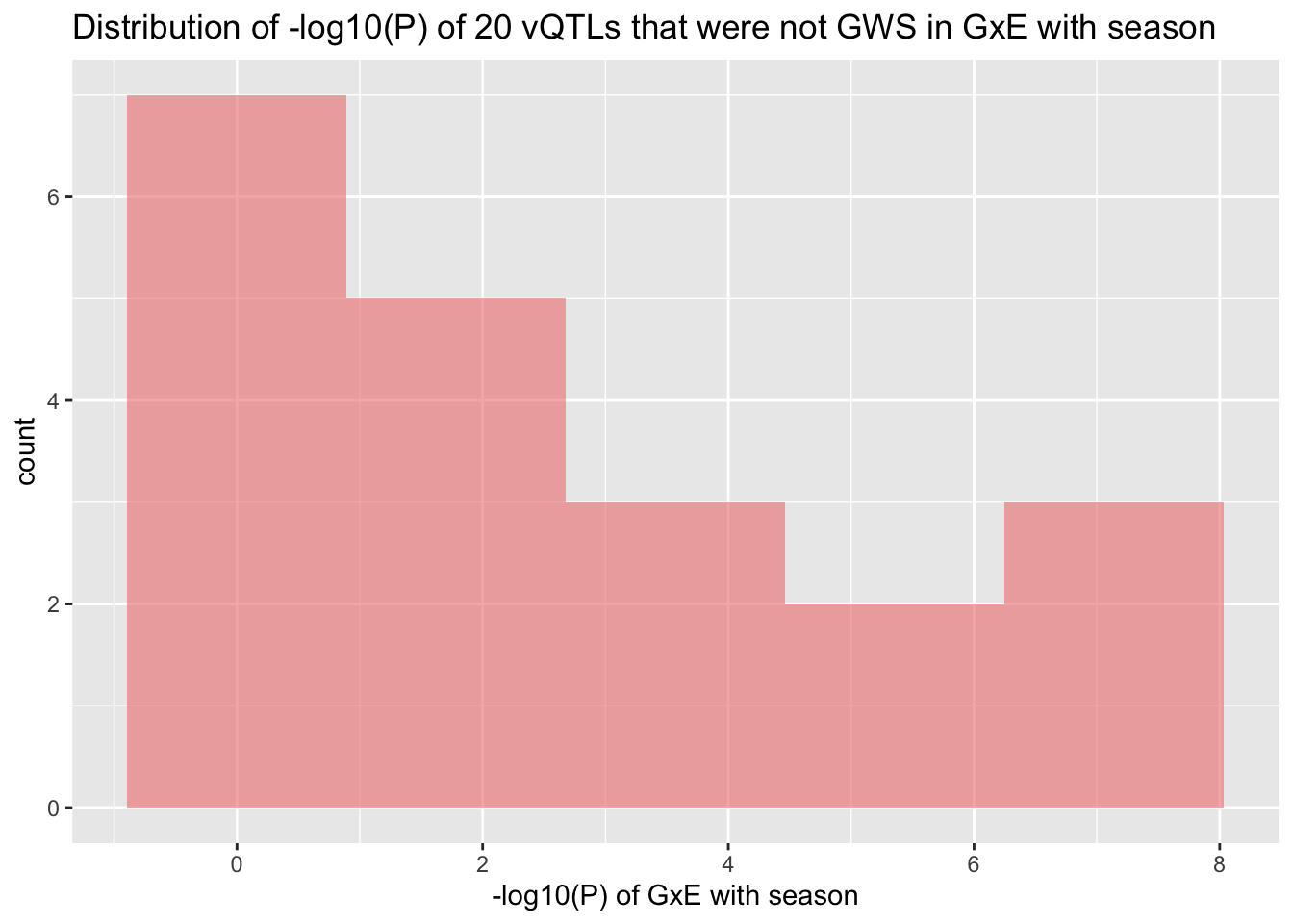
df=gxe[gxe$SNP %in% oscaGWAS_clump_common$SNP,]

# Restrict to vQTLs that are not GWS in GxE with season
df=df[df$P_GXE>5e-8,]
summary(df$P_GXE)

##      Min.   1st Qu.    Median      Mean   3rd Qu.      Max. 
## 0.0000001 0.0000517 0.0286000 0.1863237 0.2334750 0.9093000

ggplot(df, aes(-log10(P_GXE))) +
  geom_histogram(fill="lightcoral", color=alpha("grey",0), alpha=0.6, bins=5) +
  labs(title=paste0("Distribution of -log10(P) of ",nrow(df)," vQTLs that were not GWS in GxE with season"), 
       x="-log10(P) of GxE with season")

Vitamin D - vQTL GWAS