# Libraries
library(ggplot2)
library(dplyr)
library(ggrepel)
library(DT)
library(qqman)
library(gridExtra)

We hypothesised that if, for example, there were pathways involved in metabolising vitamin D (which would be active in Summer months, when vitamin D production is increased), or in storing vitamin D (which would be active in Winter months, when vitamin D production is limited), there would be different genetic variants associated with vitamin D levels in different seasons. To test that hypothesis, we stratified the UK Biobank data into two cohorts: (1) individuals assessed in Autumn/Winter, and (2) individuals assessed Spring/Summer. Then, we ran fastGWA separately in the two sub-samples. Results are presented below.

Methods

Data

The following files were used to run the analyses:

Phenotype file: File with one line per individual and a column with the phenotype. The phenotype was obtained after (1) restricting to individuals of European ancestry, (2) restricting to individuals with vitamin D levels measured in the season of interest, and (3) applying a rank-based inverse-normal transformation (RINT). Specifically, two phenotype files were used to run two GWAS (more information on Pheno page):
- “Winter” phenotype - 162591 individuals of European ancestry
- “Summer” phenotype - 177082 individuals of European ancestry
Genotype file: We restricted the analyses to individuals of European ancestry and included 44741804 autossomal variants + 260713 variants in chromosome X (including the pseudo-autosomal region). Variants had (1) MAC > 5, (2) INFO > 0.3, and (3) genotype missingness > 0.05. In addition, variants with missingness < 0.05, pHWE < 1x10^-5, and MAC > 5 in the subset of unrelated European individuals were excluded.
Sparse GRM: For this analysis we used a sparse GRM calculated using HapMap3 SNPs from individuals of European ancestry.
Covariates files: This file includes one column per covariate to fit in the model. Covariates included were: age, sex, genotyping batch, UKB assessment centre, month of assessment, information on whether vitamin supplements were ever taken, and the first 40 PCs. For more detail see the Covariates section of the Pheno page.

GWAS

We conducted two GWA analyses with Fast-GWA, restricting to SNPs with MAF>0.01.


# ------ Make mbfile with all individual-level data files to include in the analysis
tmpDir=$WD/results/stratifiedGWAS/tmpDir
genoDir=$medici/UKBiobank/v3EUR_impQC
echo $genoDir/ukbEUR_imp_chr1_v3_impQC > $tmpDir/UKB_v3EUR_impQC.files
for i in `seq 2 22`; do echo $genoDir/ukbEUR_imp_chr${i}_v3_impQC >> $tmpDir/UKB_v3EUR_impQC.files; done


# #########################################
# Run stratified GWAS - autosomes
# #########################################

# Set directories
results=$WD/results/stratifiedGWAS
tmpDir=$results/tmpDir

for season in winter summer
do
  # Files/settings to use
  prefix=vitD_${season}GWAS
  geno=$tmpDir/UKB_v3EUR_impQC.files
  pheno=$WD/input/mlm_${season}_pheno
  grm=$WD/input/UKB_HM3_m01_sp
  quantCovars=$WD/input/quantitativeCovariates
  catgCovars=$WD/input/categoricalCovariates
  snps2include=$WD/input/UKB_v3EUR_impQC/UKB_EUR_impQC_maf0.01.snplist
  output=$results/$prefix

  # Run GWAS
  cd $results
    gcta=$bin/gcta/gcta_1.92.3beta3
  tmp_command="$gcta --mbfile $geno \
                     --fastGWA-lmm \
                     --pheno $pheno \
                     --grm-sparse  $grm \
                     --qcovar $quantCovars\
                     --covar $catgCovars \
                     --covar-maxlevel 110 \
                     --extract $snps2include \
                     --threads 16 \
                     --out $output"
  qsubshcom "$tmp_command" 16 10G $prefix 24:00:00 ""
  echo $prefix
done



# Format results
for season in winter summer
do
    # Merge results from each chr after all have finished running
    prefix=vitD_${season}GWAS
    gzip $results/$prefix.fastGWA
    mv $results/$prefix.fastGWA.gz $results/$prefix.gz
    
    # Convert GWAS sumstats to .ma format (for COJO)
    echo "SNP A1 A2 freq b se p n" > $results/$prefix.ma
    zcat $results/$prefix.gz | awk '{print $2,$4,$5,$7,$8,$9,$10,$6}' | sed 1d >> $results/$prefix.ma
done


# #########################################
# Run stratified GWAS - X chromosome
# #########################################

# Set directories
results=$WD/results/stratifiedGWAS
tmpDir=$results/tmpDir

for season in winter summer
do

  # Files/settings to use
  pheno=$WD/input/mlm_${season}_pheno
  grm=$WD/input/UKB_HM3_m01_sp
  quantCovars=$WD/input/quantitativeCovariates
  catgCovars=$WD/input/categoricalCovariates_noSex

  # ---- Run GWAS separately for males and females
  cd $results
  for sex in FEMALE MALE
  do
    # Run X chromosome pseudo-autosomal region (chr XY) as well
    for region in X XY
    do
      prefix=vitD_${season}_chr$region.$sex
      geno=$medici/v3EUR_chrX/ukbEURv3_${region}_maf0.1_$sex
      output=$tmpDir/$prefix
  
      gcta=$bin/gcta/gcta_1.92.3beta3
      tmp_command="$gcta --bfile $geno \
                       --fastGWA-lmm \
                       --pheno $pheno \
                       --grm-sparse  $grm \
                       --qcovar $quantCovars\
                       --covar $catgCovars \
                       --covar-maxlevel 110 \
                       --threads 16 \
                       --out $output"
      qsubshcom "$tmp_command" 16 30G $prefix 6:00:00 ""
    done # end loop through chr
  done # end loop through sex

done # end loop through season



# #########################################
# Meta-analyse results from males and females for X and XY
# #########################################
results=$WD/results/stratifiedGWAS
tmpDir=$results/tmpDir
metal=$bin/metal/metal

# Run meta-analysis
cd $results
for season in winter summer
do

  for chr in X XY
  do
    sumstats1=$tmpDir/vitD_${season}_chr$chr.FEMALE.fastGWA
    sumstats2=$tmpDir/vitD_${season}_chr$chr.MALE.fastGWA
    output=$tmpDir/vitD_${season}_chr$chr
    METALscript=$tmpDir/$season.chr$chr.SEXmeta.METALscript
    logFile=$results/job_reports/$season.chr$chr.SEXmeta.log

    echo "
    CLEAR
    SCHEME STDERR
    AVERAGEFREQ ON

    # Describe and process results for X chromosome
    MARKER SNP
    ALLELE A1 A2
    EFFECT BETA
    PVALUE P
    WEIGHT N
    STDERR SE
    FREQLABEL AF1

    PROCESS $sumstats1
    PROCESS $sumstats2

    # Run meta-analysis
    OUTFILE $output .TBL

    ANALYZE
    " > $METALscript
    
    # Run meta-analysis
    $metal < $METALscript > $logFile

  done # end loop through chromosomes
done # end loop through seasons
    

# #########################################
# Format meta-analysed results and merge with autossomes
# Generate .ma format files for COJO
# #########################################

cd $WD/results/stratifiedGWAS
R

for(season in c("winter","summer"))
{
  prefix=paste0("vitD_",season)
  
  # Read X meta-analyses results + GWAS results for autosomes
  xmeta=read.table(paste0("tmpDir/",prefix,"_chrX1.TBL"),h=T,stringsAsFactors=F)
  xymeta=read.table(paste0("tmpDir/",prefix,"_chrXY1.TBL"),h=T,stringsAsFactors=F)
  autosomes=read.table(paste0(prefix,"GWAS.gz"), h=T,stringsAsFactors=F)
  names(xmeta)=c("SNP","A1","A2","AF1","AF1_SE","BETA","SE","P","direction")
  names(xymeta)=c("SNP","A1","A2","AF1","AF1_SE","BETA","SE","P","direction")

  # Get chrX details (BP and N) from female and male GWAS
  xfemale=read.table(paste0("tmpDir/",prefix,"_chrX.FEMALE.fastGWA"), h=T,stringsAsFactors=F)
  xmale=read.table(paste0("tmpDir/",prefix,"_chrX.MALE.fastGWA"), h=T,stringsAsFactors=F)
    ## Get all results in the same order
    xmeta=xmeta[match(xfemale$SNP,xmeta$SNP),]
    xmale=xmale[match(xfemale$SNP,xmale$SNP),]
    ## Add BP
    xmeta$POS=xfemale$POS
    # Add N
    xmeta$N=xfemale$N+xmale$N
    # Change alleles to capital letters
    xmeta$A1=toupper(xmeta$A1)
    xmeta$A2=toupper(xmeta$A2)
    # Define chromosome
    xmeta$CHR=23
    
  # Get chrXY details (BP, and N) from female and male GWAS
  xyfemale=read.table(paste0("tmpDir/",prefix,"_chrXY.FEMALE.fastGWA"), h=T,stringsAsFactors=F)
  xymale=read.table(paste0("tmpDir/",prefix,"_chrXY.MALE.fastGWA"), h=T,stringsAsFactors=F)
    ## Get all results in the same order
    xymeta=xymeta[match(xyfemale$SNP,xymeta$SNP),]
    xymale=xymale[match(xyfemale$SNP,xymale$SNP),]
    ## Add BP
    xymeta$POS=xyfemale$POS
    ## Add N
    xymeta$N=xyfemale$N+xymale$N
    # Define chromosome
    xymeta$CHR=25
    # Change alleles to capital letters
    xymeta$A1=toupper(xymeta$A1)
    xymeta$A2=toupper(xymeta$A2)

  # Make table in fastGWA format
  # CHR SNP POS A1 A2 N AF1 BETA SE P
    xmeta_fastgwa=xmeta[,c("CHR","SNP","POS","A1","A2","N","AF1","BETA","SE","P")]
    xymeta_fastgwa=xymeta[,c("CHR","SNP","POS","A1","A2","N","AF1","BETA","SE","P")]
    ## Merge X + XY + autosomes
    allChr=rbind(autosomes, xmeta_fastgwa, xymeta_fastgwa)

  # Make table in COJO (.ma) format
  # SNP A1 A2 freq b se p n
    ## CHR X
    xmeta_ma=xmeta[,c("SNP","A1","A2","AF1","BETA","SE","P","N")]
    names(xmeta_ma)=c("SNP","A1","A2","freq","b","se","p","n")
    ## CHR XY
    xymeta_ma=xymeta[,c("SNP","A1","A2","AF1","BETA","SE","P","N")]
    names(xymeta_ma)=c("SNP","A1","A2","freq","b","se","p","n")

  # Save new file formats
    ## All chromosomes
    write.table(allChr, file=gzfile(paste0(prefix,"_withX.gz")), quote=F, row.names=F)
    ## X and XY in fastGWA format (for clumping)
    write.table(xmeta_fastgwa, file=gzfile(paste0("tmpDir/",prefix,"_chrX.gz")), quote=F, row.names=F)
    write.table(xymeta_fastgwa, file=gzfile(paste0("tmpDir/",prefix,"_chrXY.gz")), quote=F, row.names=F)
    ## X and XY in .ma format (for COJO)
    write.table(xmeta_ma, paste0(prefix,"_chrX.ma"), quote=F, row.names=F)
    write.table(xymeta_ma, paste0(prefix,"_chrXY.ma"), quote=F, row.names=F)

}

COJO

The following options were used in this analysis:

–bfile: We used the GWAS individual-level genotype data as reference.
–cojo-slct: Performs a step-wise model selection of independently associated SNPs
–cojo-p 5e-8 (default): P-value to declare a genome-wide significant hit
–cojo-wind 10,000 (default): Distance (in KB) from which SNPs are considered in linkage equilibrium
–cojo-collinear 0.9 (default): maximum r2 to be considered an independent SNP, i.e. SNPs with r2>0.9 will not be considered further
–diff-freq 0.2 (default): maximum allele difference bet
extract: Restrict analysis to SNPs with MAF>0.01

# #########################################
# Run COJO on GWAS results
# #########################################

# Directories
results=$WD/results/stratifiedGWAS
tmpDir=$results/tmpDir

# Files/settings to use
random20k_dir=$WD/input/UKB_v3EURu_impQC/random20K
ldRef=$random20k_dir/ukbEURu_imp_chr{TASK_ID}_v3_impQC_random20k_maf0.01
filters=maf0.01
snps2include=$WD/input/UKB_v3EUR_impQC/UKB_EUR_impQC_$filters.snplist

for season in summer winter
do
    prefix=vitD_${season}GWAS
    inFile=$results/$prefix.ma
    outFile=$tmpDir/${prefix}_${filters}_chr{TASK_ID}

    # Run COJO
    cd $results
    gcta=$bin/gcta/gcta_1.92.3beta3
    tmp_command="$gcta --bfile $ldRef \
                       --cojo-slct \
                       --cojo-file $inFile \
                       --extract $snps2include \
                       --out ${outFile}"
                             
    qsubshcom "$tmp_command" 1 100G ${prefix}_COJO 24:00:00 "-array=1-22"
    echo ${prefix}_COJO
done




# Format results
for season in summer winter
do
    prefix=vitD_${season}GWAS
    
    # Merge COJO results once all chr finished running
    cat $tmpDir/${prefix}_${filters}*.jma.cojo | grep "Chr" | uniq > $results/${prefix}_${filters}.cojo
    cat $tmpDir/${prefix}_${filters}_chr*.jma.cojo | grep -v "Chr" |sed '/^$/d'  >> $results/${prefix}_${filters}.cojo
done

LDSC

We ran bivariate LDSC regression with both GWAS results to assess the genetic correlation between the two.

# ##############################
# Run bivariate LDSC regression
# ##############################
module load ldsc

# Directories
results=$WD/results/stratifiedGWAS
tmpDir=$results/tmpDir
ldscDir=$bin/ldsc

cd $results
for season in summer winter
do
    # Format GWAS results
    prefix=vitD_${season}GWAS
    echo "SNP A1 A2 b n p" > $tmpDir/$prefix.ldHubFormat
    awk 'NR>1 {print $1,$2,$3,$5,$8,$7}' $results/$prefix.ma >> $tmpDir/$prefix.ldHubFormat
    
    # Munge GWAS sumstats (process sumstats and restrict to HapMap3 SNPs)
    munge_sumstats.py --sumstats $tmpDir/$prefix.ldHubFormat \
                      --merge-alleles $ldscDir/w_hm3.snplist \
                      --out $tmpDir/$prefix
done

# Run rg
ldsc.py --rg  $tmpDir/vitD_winterGWAS.sumstats.gz,$tmpDir/vitD_summerGWAS.sumstats.gz \
        --ref-ld-chr $ldscDir/eur_w_ld_chr/ \
        --w-ld-chr $ldscDir/eur_w_ld_chr/ \
        --out $results/vitD_stratifiedGWAS.ldsc.rg

In addition, we ran LDSC on each GWAS (i.e. ‘Summer’ and ‘Winter’, separately), to determine proportion of phenotypic variance they explained. To run LDSC, we restricted the GWAS summary statistics to variants found in w_hm3.noMHC.snplist (downloaded from LDHub). This is a list of HapMap3 SNPs and excludes SNPs in the MHC region.

module load ldsc

# Directories
results=$WD/results/stratifiedGWAS
tmpDir=$results/tmpDir
ldscDir=$bin/ldsc

cd $results
for season in summer winter
do
  # Format GWAS results
  prefix=vitD_${season}GWAS
  awk '{print $1,$2,$3,$5,$8,$7}' $results/$prefix.ma > $tmpDir/$prefix.ldHubFormat

  # Restrict to common SNPs
  sed 1q $tmpDir/$prefix.ldHubFormat > $results/$prefix.ldHubFormat
  awk 'NR==FNR{a[$1];next} ($1 in a)' $WD/input/UKB_v3EURu_impQC/UKB_EURu_impQC_maf0.01.snplist <(awk 'NR==FNR{a[$1];next} ($1 in a)' $WD/input/w_hm3.noMHC.snplist $tmpDir/$prefix.ldHubFormat) >> $results/$prefix.ldHubFormat

  # Munge sumstats (process sumstats and restrict to HapMap3 SNPs)
  munge_sumstats.py --sumstats $results/$prefix.ldHubFormat \
                    --merge-alleles $ldscDir/w_hm3.snplist \
                    --out $tmpDir/$prefix

  # Run LDSC
  ldsc.py --h2 $tmpDir/$prefix.sumstats.gz \
          --ref-ld-chr $ldscDir/eur_w_ld_chr/ \
          --w-ld-chr $ldscDir/eur_w_ld_chr/ \
          --out $results/$prefix.ldsc
done

Results

Note: All results presented are for variants with MAF>0.01.

Genetic correlation

# Read-in bivariate LDSC regression results
tmp=read.table("results/stratifiedGWAS/vitD_stratifiedGWAS.ldsc.rg.log", skip=30, fill=T, h=F, colClasses="character", sep="_")[,1]

# Get results:
intercept=strsplit(grep("Intercept",tmp, value=T)[3],":")[[1]][2]
rg=strsplit(grep("Genetic Correlation:",tmp, value=T),":")[[1]][2]

We ran bivariate LDSC regression with both GWAS results to assess the genetic correlation between the two:

Bivariate LDSC Intercept: 0.011 (0.0189)
Genetic Correlation: 0.8941 (0.0517)

The genetic correlation between the two traits is high, indicating that the genetic background associated with vitamin D levels in winter is similar to the genetic background associated with vitamin D levels in summer.

Manhattan plot

Summer GWAS

# Read in GWAS results ---------------------------
#gwas=read.table("results/stratifiedGWAS/vitD_summer_withX.gz", h=T, stringsAsFactors=F)
#saveRDS(gwas, file="results/stratifiedGWAS/vitD_summer_withX.RDS")
gwas=readRDS("results/stratifiedGWAS/vitD_summer_withX.RDS")
names(gwas)[grep("POS",names(gwas))]="BP"
cojo=read.table("results/stratifiedGWAS/vitD_summerGWAS_maf0.01.cojo", h=T, stringsAsFactors=F)


# Add cumulative position + clumping/cojo information for plotting
  # ----- Add chromosome start site to the GWAS result
  don=aggregate(BP~CHR,gwas,max)
  don$tot=cumsum(as.numeric(don$BP))-don$BP
  don=merge(gwas,don[,c("CHR","tot")])
  # ----- Add a cumulative position to plot in this order
  don=don[order(don$CHR,don$BP),]
  # ----- Restrict SNPs with P<0.03 + a random samples of 100K SNPs (to plot faster)
  don=don[don$P<0.03 | don$SNP %in% sample(gwas$SNP,100000),]
  don$BPcum=don$BP+don$tot
  # ----- Add cojo information
  don$is_cojo_sig=ifelse(don$SNP %in% cojo$SNP & don$P<1e-15, "yes","no")
  don$is_cojo_nonSig=ifelse(don$SNP %in% cojo$SNP & don$P>5e-8, "yes","no")
  don$is_cojo=ifelse(don$SNP %in% cojo$SNP, "yes","no")

  # ----- Prepare X axis
  axisdf = don %>% group_by(CHR) %>% summarize(center=( max(BPcum) + min(BPcum) ) / 2 )
  
  
# Generate Manhattan plot
ggplot(don, aes(x=BPcum, y=-log10(P))) +
    geom_point( aes(color=as.factor(CHR)), alpha=0.3, size=0.5) +
    scale_color_manual(values = rep(c("lightsteelblue4", "lightsteelblue3"),44)) +
    # Highlighted SNPs of interest
    geom_point(data=don[don$is_cojo=="yes",], color="red", size=2) +
    geom_label_repel( data=don[don$is_cojo_sig=="yes",], aes(label=SNP), size=2) +
    # Make X axis
    scale_x_continuous( label=axisdf$CHR, breaks=axisdf$center ) +
    labs(x="")+
    theme_bw() +
    theme(legend.position="none",
          panel.border = element_blank(),
          panel.grid.major.x = element_blank(),
          panel.grid.minor.x = element_blank())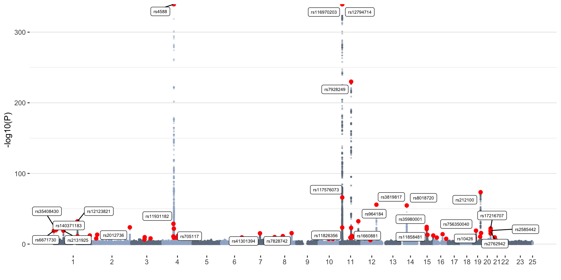

# Keep info to summarise in the report below
summer_common=gwas
summer_cojo_common=cojo

Red dots represent independent associations identified with COJO. Top independent SNPs (P<1x10^-15) are labeled.

Winter GWAS

# Read in GWAS results ---------------------------
#gwas=read.table("results/stratifiedGWAS/vitD_winter_withX.gz", h=T, stringsAsFactors=F)
#saveRDS(gwas, "results/stratifiedGWAS/vitD_winter_withX.RDS")
gwas=readRDS("results/stratifiedGWAS/vitD_winter_withX.RDS")
names(gwas)[grep("POS",names(gwas))]="BP"
cojo=read.table("results/stratifiedGWAS/vitD_winterGWAS_maf0.01.cojo", h=T, stringsAsFactors=F)


# Add cumulative position + clumping/cojo information for plotting
  # ----- Add chromosome start site to the GWAS result
  don=aggregate(BP~CHR,gwas,max)
  don$tot=cumsum(as.numeric(don$BP))-don$BP
  don=merge(gwas,don[,c("CHR","tot")])
  # ----- Add a cumulative position to plot in this order
  don=don[order(don$CHR,don$BP),]
  # ----- Restrict SNPs with P<0.03 + a random samples of 100K SNPs (to plot faster)
  don=don[don$P<0.03 | don$SNP %in% sample(gwas$SNP,100000),]
  don$BPcum=don$BP+don$tot
  # ----- Add cojo information
  don$is_cojo_sig=ifelse(don$SNP %in% cojo$SNP & don$P<1e-15, "yes","no")
  don$is_cojo_nonSig=ifelse(don$SNP %in% cojo$SNP & don$P>5e-8, "yes","no")
  don$is_cojo=ifelse(don$SNP %in% cojo$SNP, "yes","no")

  # ----- Prepare X axis
  axisdf = don %>% group_by(CHR) %>% summarize(center=( max(BPcum) + min(BPcum) ) / 2 )
  
  
# Generate Manhattan plot
ggplot(don, aes(x=BPcum, y=-log10(P))) +
    geom_point( aes(color=as.factor(CHR)), alpha=0.3, size=0.5) +
    scale_color_manual(values = rep(c("lightsteelblue4", "lightsteelblue3"),44)) +
    # Highlighted SNPs of interest
    geom_point(data=don[don$is_cojo=="yes",], color="red", size=2) +
    geom_label_repel( data=don[don$is_cojo_sig=="yes",], aes(label=SNP), size=2) +
    # Make X axis
    scale_x_continuous( label=axisdf$CHR, breaks=axisdf$center ) +
    labs(x="")+
    theme_bw() +
    theme(legend.position="none",
          panel.border = element_blank(),
          panel.grid.major.x = element_blank(),
          panel.grid.minor.x = element_blank())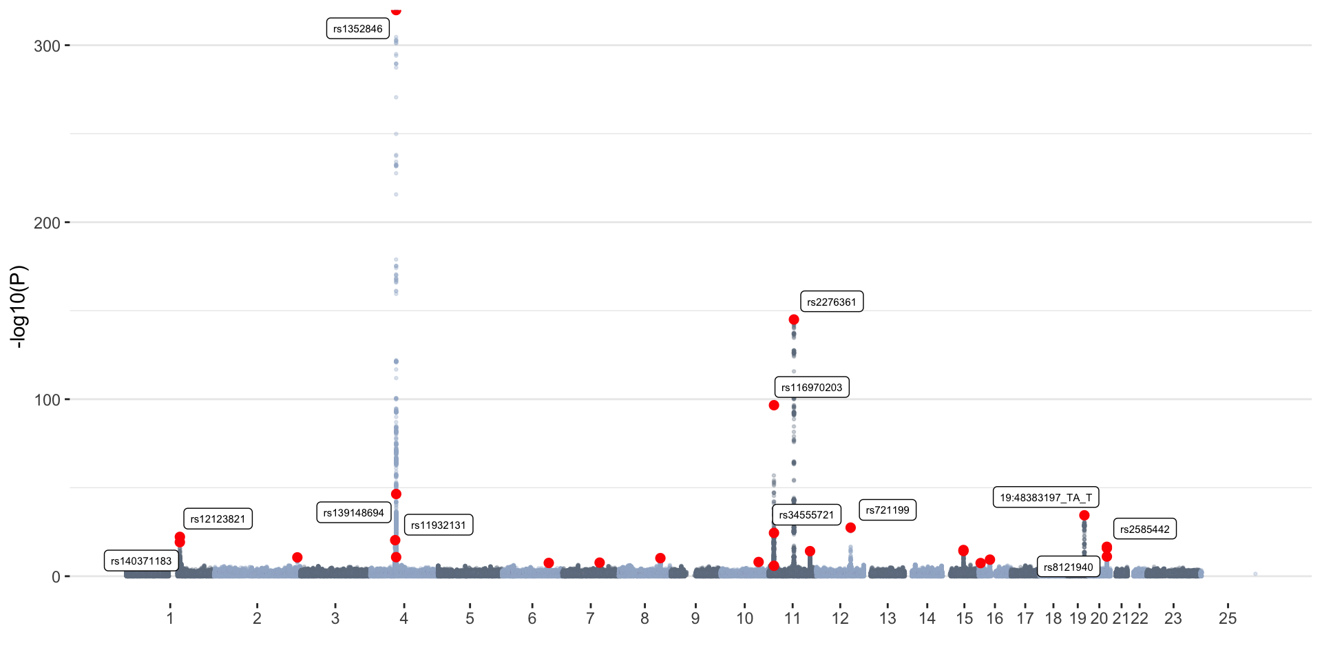

# Keep info to summarise in the report below
winter_common=gwas
winter_cojo_common=cojo

Red dots represent independent associations identified with COJO. Top independent SNPs (P<1x10^-15) are labeled.

Summary of results

Summer GWAS

8806780 variants tested
12331 GWS (P<5x10^-8) hits
70 independent associations (determined with COJO)
65 independent associations (determined with COJO) that were GWS in the original GWAS

indep = summer_cojo_common %>% arrange(Chr, bp)

# Format table
indep=indep[,c("Chr","SNP","bp","refA","freq","b","se","p","n","freq_geno","bJ","bJ_se","pJ")]
indep$p=format(indep$p, digits=3)
indep$pJ=format(indep$pJ, digits=3)
indep=indep %>% mutate_at(vars(se, bJ_se, b, bJ), round, 4)
indep=indep %>% mutate_at(vars(freq, freq_geno), round, 2)

# Present table
datatable(indep, 
          rownames=FALSE, 
          extensions=c('Buttons','FixedColumns'),
          options=list(pageLength=5,
                       dom='frtipB',
                       buttons=c('csv', 'excel'),
                       scrollX=TRUE),
          caption="List of independent associations in summer GWAS") %>% 
  formatStyle("p","white-space"="nowrap") %>% 
  formatStyle("pJ","white-space"="nowrap")

Columns are: Chr, chromosome; SNP, SNP rs ID; bp, physical position; refA, the effect allele; type, type of QTL; freq, frequency of the effect allele in the original data; b, se and p, effect size, standard error and p-value from the original GWAS; n, estimated effective sample size; freq_geno, frequency of the effect allele in the reference sample; bJ, bJ_se and pJ, effect size, standard error and p-value from a joint analysis of all the selected SNPs.

Winter GWAS

8806780 variants tested
3993 GWS (P<5x10^-8) hits
26 independent associations (determined with COJO)
25 independent associations (determined with COJO) that were GWS in the original GWAS

indep = winter_cojo_common %>% arrange(Chr, bp)

# Format table
indep=indep[,c("Chr","SNP","bp","refA","freq","b","se","p","n","freq_geno","bJ","bJ_se","pJ")]
indep$p=format(indep$p, digits=3)
indep$pJ=format(indep$pJ, digits=3)
indep=indep %>% mutate_at(vars(se, bJ_se, b, bJ), round, 4)
indep=indep %>% mutate_at(vars(freq, freq_geno), round, 2)


# Present table
datatable(indep, 
          rownames=FALSE, 
          extensions=c('Buttons','FixedColumns'),
          options=list(pageLength=5,
                       dom='frtipB',
                       buttons=c('csv', 'excel'),
                       scrollX=TRUE),
          caption="List of independent associations in winter GWAS") %>% 
  formatStyle("p","white-space"="nowrap") %>% 
  formatStyle("pJ","white-space"="nowrap")

QQplot + LDSC

Summer GWAS

gwas=summer_common
names(gwas)[grep("p",names(gwas))]="P"

pthrh=0.03
tmp=c(gwas[gwas$P<pthrh,"P"], sample(gwas[gwas$P>pthrh,"P"],100000))

qq(tmp)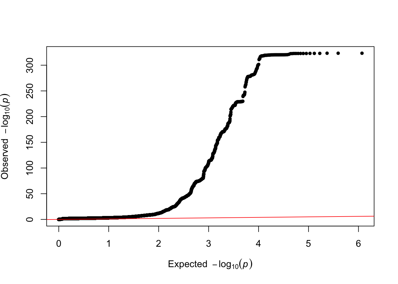

LDSC

tmp=read.table("results/stratifiedGWAS/vitD_summerGWAS.ldsc.log", skip=15, fill=T, h=F, colClasses="character", sep="_")[,1]

# Get results:
h2=strsplit(grep("Total Observed scale h2",tmp, value=T),":")[[1]][2]
lambda_gc=strsplit(grep("Lambda GC",tmp, value=T),":")[[1]][2]
chi2=strsplit(grep("Mean Chi",tmp, value=T),":")[[1]][2]
intercept=strsplit(grep("Intercept",tmp, value=T),":")[[1]][2]
ratio=strsplit(grep("Ratio",tmp, value=T),":")[[1]][2]

Total Observed scale h²: 0.1389 (0.0293)
Lambda GC: 1.2564
Mean Chi²: 1.5253
Intercept: 1.0263 (0.0119)
Ratio: 0.05 (0.0226)

Winter GWAS

gwas=winter_common
names(gwas)[grep("p",names(gwas))]="P"
pthrh=0.03
tmp=c(gwas[gwas$P<pthrh,"P"], sample(gwas[gwas$P>pthrh,"P"],100000))

pw=qq(tmp)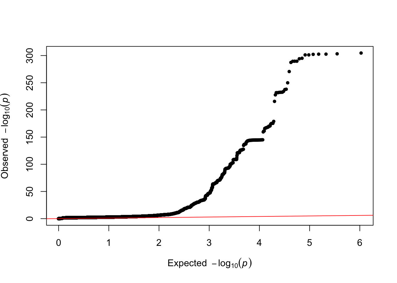

LDSC

tmp=read.table("results/stratifiedGWAS/vitD_winterGWAS.ldsc.log", skip=15, fill=T, h=F, colClasses="character", sep="_")[,1]

# Get results:
h2=strsplit(grep("Total Observed scale h2",tmp, value=T),":")[[1]][2]
lambda_gc=strsplit(grep("Lambda GC",tmp, value=T),":")[[1]][2]
chi2=strsplit(grep("Mean Chi",tmp, value=T),":")[[1]][2]
intercept=strsplit(grep("Intercept",tmp, value=T),":")[[1]][2]
ratio=strsplit(grep("Ratio",tmp, value=T),":")[[1]][2]

Total Observed scale h²: 0.0862 (0.0134)
Lambda GC: 1.1973
Mean Chi²: 1.2942
Intercept: 1.0167 (0.0088)
Ratio: 0.0569 (0.0298)

Vitamin D - Season-stratified GWAS

Methods

Data

GWAS

COJO

LDSC

Results

Genetic correlation

Manhattan plot

Summer GWAS

Winter GWAS

Summary of results

Summer GWAS

Winter GWAS

QQplot + LDSC

Summer GWAS

Winter GWAS