Relationship with BMI
# Libraries
library(ggplot2)
library(dplyr)
library(ggrepel)
library(DT)
library(qqman)
library(kableExtra)
library(gridExtra)
library(limma)
library(ggforce)
BMI has previously been reported to associate with vitamin D levels. However, to prevent collider bias, we did not include BMI as a covariate in our GWAS.
Here, we assessed the relationship between BMI and vitamin D. For this, we used GWA results for BMI presented in Xue et al. 2018 Nat Commun. First, we assessed the genetic correlation between vitamin D and BMI. Second, we used generalised summary-data-based Mendelian randomisation (GSMR) to test for putative causal effects between the two traits. Third, we performed a multi-trait-based conditional & joint analysis (mtCOJO) to condition the vitamin D GWAS on BMI and estimate its effect on vitamin D.
Methods
Genetic correlation
We calculated the genetic correlation between vitamin D and BMI using LDSC regression. We restricted this analysis to a list of HapMap3 SNPs with no variants in the MHC region. The list of SNPs (w_hm3.noMHC.snplist) was downloaded from LDHub.
# Get BMI GWAS susmstats
# From Xue, A. et al. Genome-wide association analyses identify 143 risk variants and putative regulatory mechanisms for type 2 diabetes. Nat. Commun. 9, 2941 (2018).


# ##############################
# Run bivariate LDSC regression
# ##############################

#  ------ Using UKB BMI sumstats
module load ldsc
prefix=vitD_fastGWA
bmi_prefix=ukbBMI

# Directories
results=$WD/results/fastGWA
tmpDir=$results/tmpDir
ldscDir=$bin/ldsc

# Format BMI GWAS results
echo "SNP A1 A2 b n p" > $WD/input/gwas_sumstats/1_LDSRFormat/$bmi_prefix.ldHubFormat
awk 'NR>1 {print $2,$4,$5,$8,$7,$10}' $WD/input/gwas_sumstats/0_original/ukbEUR_BMI_common.txt >> $WD/input/gwas_sumstats/1_LDSRFormat/$bmi_prefix.ldHubFormat

# Munge (process sumstats and restrict to HapMap3 SNPs) BMI sumstats
munge_sumstats.py --sumstats $WD/input/gwas_sumstats/1_LDSRFormat/$bmi_prefix.ldHubFormat \
                  --merge-alleles $ldscDir/w_hm3.snplist \
                  --out  $WD/input/gwas_sumstats/2_LDSRMungeFormat/$bmi_prefix

# Run rg
ldsc.py --rg  $results/ldscFormat/$prefix.sumstats.gz,$WD/input/gwas_sumstats/2_LDSRMungeFormat/$bmi_prefix.sumstats.gz\
        --ref-ld-chr $ldscDir/eur_w_ld_chr/ \
        --w-ld-chr $ldscDir/eur_w_ld_chr/ \
        --out $results/ldsc/$prefix.$bmi_prefix.ldsc.rg
GSMR
We performed bi-directional GSMR on BMI and vitamin D with the GCTA-implemented GSMR method. The following options were used:
- –mbfile: We used a random subset of 20,000 unrelated individuals of European ancestry from the UKB as LD reference (same as previously used for COJO analyses)
- –gsmr-file: The two GWAS used in the analysis:
- Vitamin D fastGWA results (presented in GWAS section)
- BMI GWAS results by Xue et al. 2018 Nat Commun (PMID 30054458)
- –gsmr-direction: We ran bi-directoial GSMR analysis (coded as 2)
- –gsmr-snp-min 10 (default): Minimum number of GW significant and near-independent SNPs required for the GSMR analysis.
- –gwas-thresh 5e-8 (default): P-value threshold to select SNPs for clumping.
prefix=vitD_fastGWA
bmi_prefix=ukbBMI

# Directories
results=$WD/results/fastGWA
tmpDir=$results/tmpDir
gwasDir=$WD/input/gwas_sumstats
random20k_dir=$WD/input/UKB_v3EURu_impQC/random20K


# ########################
# Prepare files to run GSMR
# ########################

# --- Create file with paths to LD reference data
#     Use random set of 20K unrelated Europeans previously extracted for COJO analysis
  echo $random20k_dir/ukbEURu_imp_chr1_v3_impQC_random20k_maf0.01 > $tmpDir/ukb_ref_data.txt
  for i in `seq 2 22`; do echo $random20k_dir/ukbEURu_imp_chr${i}_v3_impQC_random20k_maf0.01 >> $tmpDir/ukb_ref_data.txt; done


# --- Convert BMI results to .ma format, remove duplicated SNPs and create file with name and path to that file
  echo "SNP A1 A2 freq b se p N" > $gwasDir/3_maFormat/$bmi_prefix.ma
  awk 'NR>1 {print $2,$4,$5,$6,$8,$9,$10,$7}' $gwasDir/0_original/ukbEUR_BMI_common.txt | awk '!seen[$1]++'>> $gwasDir/3_maFormat/$bmi_prefix.ma
  echo "bmi $gwasDir/3_maFormat/$bmi_prefix.ma" > $tmpDir/files4gsmr.bmi

# --- Create file with name and path to vitamin D results
echo "vitD $results/maFormat/$prefix.ma" > $tmpDir/files4gsmr.vitD


# ########################
# Run bi-directional GSMR
# ########################

# Files/settings to use
ld_ref=$tmpDir/ukb_ref_data.txt
ids2keep=$medici/v3Samples/ukbEURu_v3_all_20K.fam
exposure=$tmpDir/files4gsmr.bmi
outcome=$tmpDir/files4gsmr.vitD

# Run GSMR without HEIDI
cd $results
gcta=$bin/gcta/gcta_1.92.3beta3
output=$results/gsmr/$prefix.$bmi_prefix.gsmr_with20kUKB_noHeidi
tmp_command="$gcta --mbfile $ld_ref  \
                   --gsmr-file $exposure $outcome \
                   --gsmr-direction 2 \
                   --heidi-thresh 0  \
                   --effect-plot \
                   --gsmr-snp-min 10 \
                   --gwas-thresh 5e-8 \
                   --threads 16  \
                   --out $output"
qsubshcom "$tmp_command" 16 30G $(basename $output) 24:00:00 ""


# Run GSMR with new HEIDI-outlier method
cd $results
gcta=$bin/gcta/gcta_1.92.3beta3
output=$results/gsmr/$prefix.$bmi_prefix.gsmr_with20kUKB_2heidi
tmp_command="$gcta --mbfile $ld_ref  \
                   --keep  $ids2keep \
                   --gsmr-file $exposure $outcome \
                   --gsmr-direction 2 \
                   --effect-plot \
                   --gsmr-snp-min 10 \
                   --gwas-thresh 5e-8 \
                   --gsmr2-beta  \
                   --heidi-thresh  0.01 0.01  \
                   --threads 16  \
                   --out $output"
qsubshcom "$tmp_command" 16 30G $(basename $output) 24:00:00 ""


# ##############################################
# Run bi-directional GSMR with pleiotropic SNPs
# ##############################################

# --------- Generate lists of pleiotropic SNPs to use in the analyses

# BMI pleiotropic SNPs
bmi_pleioSNPs=$tmpDir/$bmi_prefix.$prefix.pleioSNPs
awk 'NR==1' $results/gsmr/$prefix.$bmi_prefix.gsmr_with20kUKB_2heidi.pleio_snps | awk '{print $3}' | tr ',' '\n' > $bmi_pleioSNPs

# Vitamin D pleiotropic SNPs
vitD_pleioSNPs=$tmpDir/$prefix.$bmi_prefix.pleioSNPs
awk 'NR==2' $results/gsmr/$prefix.$bmi_prefix.gsmr_with20kUKB_2heidi.pleio_snps | awk '{print $3}' | tr ',' '\n' > $vitD_pleioSNPs

# -------- Run GSMR

# Files/settings to use
ld_ref=$tmpDir/ukb_ref_data.txt
exposure=$tmpDir/files4gsmr.bmi
outcome=$tmpDir/files4gsmr.vitD

# Run GSMR without HEIDI - with BMI pleiotropic SNPs
cd $results
gcta=$bin/gcta/gcta_1.92.3beta3
output=$results/gsmr/gsmr_with20kUKB_noHeidi.$prefix.$bmi_prefix.bmi_pleioSNPs
tmp_command="$gcta --mbfile $ld_ref  \
                   --gsmr-file $exposure $outcome \
                   --gsmr-direction 0 \
                   --heidi-thresh 0  \
                   --extract $bmi_pleioSNPs \
                   --effect-plot \
                   --gsmr-snp-min 10 \
                   --gwas-thresh 5e-8 \
                   --threads 16  \
                   --out $output"
qsubshcom "$tmp_command" 16 30G $(basename $output) 24:00:00 ""

# Run GSMR without HEIDI - with vitamin D pleiotropic SNPs
cd $results
gcta=$bin/gcta/gcta_1.92.3beta3
output=$results/gsmr/gsmr_with20kUKB_noHeidi.$prefix.$bmi_prefix.vitD_pleioSNPs
tmp_command="$gcta --mbfile $ld_ref  \
                   --gsmr-file $exposure $outcome \
                   --gsmr-direction 1 \
                   --heidi-thresh 0  \
                   --extract $vitD_pleioSNPs \
                   --effect-plot \
                   --gsmr-snp-min 10 \
                   --gwas-thresh 5e-8 \
                   --threads 16  \
                   --out $output"
qsubshcom "$tmp_command" 16 30G $(basename $output) 24:00:00 ""
In addition, we ran bi-directional GSMR with BMI and BMI-conditioned vitamin D obtained with mtCOJO.
mtCOJO
We conducted a mtCOJO analysis to condition the vitamin D GWAS on the BMI GWAS results.
prefix=vitD_fastGWA
bmi_prefix=ukbBMI

# Directories
results=$WD/results/fastGWA
tmpDir=$results/tmpDir
ldscDir=$bin/ldsc
gwasDir=$WD/input/gwas_sumstats/3_maFormat

# ########################
# Prepare files to run mtCOJO
# ########################

# Vitamin D conditioned on BMI
echo "vitD $results/maFormat/$prefix.ma
bmi $gwasDir/$bmi_prefix.ma" > $tmpDir/files4mtCOJO.${prefix}_condition_on_$bmi_prefix

# BMI conditioned on vitamin D
echo "bmi $gwasDir/$bmi_prefix.ma
vitD $results/maFormat/$prefix.ma" > $tmpDir/files4mtCOJO.${bmi_prefix}_condition_on_$prefix

# ########################
# Run mtCOJO
# ########################

# Files/settings to use
ld_ref=$tmpDir/ukb_ref_data.txt
ids2keep=$medici/v3Samples/ukbEURu_v3_all_20K.fam
ldscFiles=$ldscDir/eur_w_ld_chr/
analysis=${prefix}_condition_on_$bmi_prefix
#analysis=${bmi_prefix}_condition_on_$prefix
gwasDatasets=$tmpDir/files4mtCOJO.$analysis
output=$results/mtcojo.$analysis

# Run mtCOJO
cd $results
gcta=$bin/gcta/gcta_1.92.3beta3
tmp_command="$gcta --mbfile $ld_ref  \
                   --keep $ids2keep \
                   --mtcojo-file $gwasDatasets \
                   --ref-ld-chr $ldscFiles \
                   --w-ld-chr $ldscFiles \
                   --threads 16  \
                   --out $output"
qsubshcom "$tmp_command" 16 30G $(basename $output) 24:00:00 ""

# Convert results to .ma format (for COJO, mtCOJO and SMR)
  echo "SNP A1 A2 freq b se p n" > $results/maFormat/`basename $output`.ma
  awk 'NR>1 {print $1,$2,$3,$4,$9,$10,$11,$8}' $output.mtcojo.cma | awk '!seen[$1]++' >>  $results/maFormat/`basename $output`.ma
  ln -s $results/maFormat/mtcojo.vitD_fastGWA_condition_on_ukbBMI.ma $results/maFormat/vitD_BMIcond_fastGWA.ma

# Convert results to fastGWA format (to upload to FUMA - need CHR and BP)
  posFile=read.table("input/UKB_v3EURu_impQC/v3EURu_impQC.bim", h=F, stringsAsFactors=F, col.names=c("CHR","SNP","MG","BP","A1","A2"))
  sumstats=read.table("results/fastGWA/mtcojo.vitD_fastGWA_condition_on_ukbBMI.mtcojo.cma", h=T, stringsAsFactors=F)
  tmp=merge(posFile[,c("CHR","SNP","BP")], sumstats, all.y=T)
  tmp=tmp[,c("CHR","SNP","BP","A1","A2","N","freq","bC","bC_se","bC_pval")]
  names(tmp)=c("CHR","SNP","POS","A1","A2","N","AF1","BETA","SE","P")
  write.table(tmp, file=gzfile("results/fastGWA/vitD_BMIcond_fastGWA.gz"), row.names=F, quote=F)
Then, we re-ran GSMR on the BMI-conditioned vitamin D GWAS (mtCOJO) results.
prefix=vitDmtcojo
bmi_prefix=ukbBMI

# Directories
results=$WD/results/fastGWA
tmpDir=$results/tmpDir
ldscDir=$bin/ldsc


# ########################
# Prepare files to run GSMR
# ########################

# Create a file with name and path to mtCOJO results in .ma format
echo "vitD_bmi_mtcojo $results/maFormat/mtcojo.vitD_fastGWA_condition_on_ukbBMI.ma" > $tmpDir/files4gsmr.vitDmtcojo


# ########################
# Run bi-directional GSMR
# ########################

# Files/settings to use
ld_ref=$tmpDir/ukb_ref_data.txt
exposure=$tmpDir/files4gsmr.bmi
outcome=$tmpDir/files4gsmr.vitDmtcojo

# Run GSMR without HEIDI
cd $results
gcta=$bin/gcta/gcta_1.92.3beta3
output=$results/gsmr/gsmr_with20kUKB_noHeidi_$prefix.$bmi_prefix
tmp_command="$gcta --mbfile $ld_ref  \
                   --gsmr-file $exposure $outcome \
                   --gsmr-direction 2 \
                   --heidi-thresh 0  \
                   --effect-plot \
                   --gsmr-snp-min 10 \
                   --gwas-thresh 5e-8 \
                   --threads 16  \
                   --out $output"
qsubshcom "$tmp_command" 16 30G $(basename $output) 24:00:00 ""


# Run GSMR with new HEIDI-outlier method
cd $results
gcta=$bin/gcta/gcta_1.92.3beta3
output=$results/gsmr/gsmr_with20kUKB_2heidi_$prefix.$bmi_prefix
tmp_command="$gcta --mbfile $ld_ref  \
                   --gsmr-file $exposure $outcome \
                   --gsmr-direction 2 \
                   --effect-plot \
                   --gsmr-snp-min 10 \
                   --gwas-thresh 5e-8 \
                   --gsmr2-beta  \
                   --heidi-thresh  0.01 0.01  \
                   --threads 16  \
                   --out $output"
qsubshcom "$tmp_command" 16 30G $(basename $output) 24:00:00 ""
Lastly, we conducted COJO analysis on the mtCOJO results to identify the set of independent variants that had a jointly significant association with vitamin D after conditioning on BMI. The following options were used to run COJO:
- –bfile: We used a random subset of 20,000 unrelated individuals of European ancestry from the UKB as LD reference (same as previously used for COJO analyses)
- –cojo-slct: Performs a step-wise model selection of independently associated SNPs
- –cojo-p 5e-8 (default): P-value to declare a genome-wide significant hit
- –cojo-wind 10,000: Distance (in KB) from which SNPs are considered in linkage equilibrium
- –cojo-collinear 0.9 (default): maximum r2 to be considered an independent SNP, i.e. SNPs with r2>0.9 will not be considered further
- –diff-freq 0.2 (default): maximum allele difference between the GWAS and the LD reference sample
- extract: Restrict analysis to SNPs with MAF>0.01
# ########################
# Run COJO on mtCOJO results
# ########################

prefix=mtcojo.vitD_fastGWA_condition_on_ukbBMI

# Directories
results=$WD/results/fastGWA
tmpDir=$results/tmpDir
random20k_dir=$WD/input/UKB_v3EURu_impQC/random20K

# Files/settings
ldRef=$random20k_dir/ukbEURu_imp_chr{TASK_ID}_v3_impQC_random20k_maf0.01
inFile=$results/maFormat/$prefix.ma
filters=maf0.01
snps2include=$WD/input/UKB_v3EUR_impQC/UKB_EUR_impQC_$filters.snplist
outFile=$tmpDir/$prefix.$filters.chr{TASK_ID}

# Run COJO
cd $results
gcta=$bin/gcta/gcta_1.92.3beta3
tmp_command="$gcta --bfile $ldRef \
                   --cojo-slct \
                   --cojo-file $inFile \
                   --extract $snps2include \
                   --out $outFile"
qsubshcom "$tmp_command" 1 60G COJO.$prefix 24:00:00 "-array=1-22"

# Merge COJO results once all chr finished running
cat $tmpDir/$prefix.$filters*.jma.cojo | grep "Chr" | uniq > $results/$prefix.cojo
cat $tmpDir/$prefix.$filters*.jma.cojo | grep -v "Chr" |sed '/^$/d'  >> $results/$prefix.cojo
2SMR
In addition to GSMR, we perfomed MR analyses between 25OHD and BMI using 2-sample MR.
# #########################################
# Generate table with all combinations of exposure and outcome GWAS to run 2SMR with
# #########################################
WD=getwd()

# Details of vitamin D GWAS
exposureList=data.frame(Trait="vitD",
                        FilePath=paste0(WD,"/results/fastGWA/maFormat/vitD_fastGWA_withX.ma"),
                        stringsAsFactors=F)

# Details of other trait GWAS
outcomeList=data.frame(Trait="ukbBMI",
                       FilePath=paste0(WD,"/input/gwas_sumstats/3_maFormat/ukbBMI.ma"))

# Combine in one table
df=cbind(exposureList, outcomeList)
tmp=cbind(outcomeList, exposureList)
df=rbind(df,tmp)
names(df)=c("exposure","exposureFile","outcome","outcomeFile")
df$heidi="noHeidi"
tmp=df
tmp$heidi="withHeidi"
df=rbind(df,tmp)
df[grep("vitD", df$exposure),"direction"]="12"
df[grep("vitD", df$outcome),"direction"]="21"

# Save table
write.table(df, "results/fastGWA/twosmr/input/analyses2run_ukbBMI", quote=F, row.names=F)
# #########################################
# Extract instruments from GSMR analyses
# #########################################
results=$WD/results/fastGWA
tmpDir=$results/tmpDir
exposure=ukbBMI
outcome=vitD
# Get lists of instruments used in both directions - no HEIDI
heidi=noHeidi
gsmr_log=$results/gsmr/vitD_fastGWA.ukbBMI.gsmr_with20kUKB_noHeidi.eff_plot.gz
zcat $gsmr_log | tail -4 | sed 1q | tr ' ' '\n' > $tmpDir/gsmr_with20kUKB_${heidi}_$exposure.$outcome.gsmr12instruments
zcat $gsmr_log | tail -2 | sed 1q | tr ' ' '\n' > $tmpDir/gsmr_with20kUKB_${heidi}_$exposure.$outcome.gsmr21instruments
# Get lists of instruments used in both directions - with HEIDI
heidi=withHeidi
gsmr_log=$results/gsmr/vitD_fastGWA.ukbBMI.gsmr_with20kUKB_2heidi.eff_plot.gz
zcat $gsmr_log | tail -4 | sed 1q | tr ' ' '\n' > $tmpDir/gsmr_with20kUKB_${heidi}_$exposure.$outcome.gsmr12instruments
zcat $gsmr_log | tail -2 | sed 1q | tr ' ' '\n' > $tmpDir/gsmr_with20kUKB_${heidi}_$exposure.$outcome.gsmr21instruments
# #########################################
# Submit 2SMR jobs
# #########################################
results=$WD/results/fastGWA
analyses2run=$results/twosmr/input/analyses2run_ukbBMI
n=`wc -l < $analyses2run`
cd $results
if test $n != 1; then arrays="-array=2-$n"; i="{TASK_ID}"; else arrays=""; i=1; fi
get_inputParameters="exposure=\$(awk -v i=$i 'NR==i {print \$1}' $analyses2run);
outcome=\$(awk -v i=$i 'NR==i {print \$3}' $analyses2run);
exposure_GWASfile=\$(awk -v i=$i 'NR==i {print \$2}' $analyses2run);
outcome_GWASfile=\$(awk -v i=$i 'NR==i {print \$4}' $analyses2run);
direction=\$(awk -v i=$i 'NR==i {print \$6}' $analyses2run);
heidi=\$(awk -v i=$i 'NR==i {print \$5}' $analyses2run)"
run2smr="Rscript $WD/scripts/run2smr.R $WD
\$exposure
\$outcome \
\$exposure_GWASfile
\$outcome_GWASfile \
\$direction
\$heidi"
qsubshcom "$get_inputParameters; $run2smr" 1 30G run2smr 5:00:00 "$arrays"
# Merge results
sed 1q $results/twosmr/*ukbBMI*2smr | uniq | tr ' ' '\t' > $results/twosmr/ukbBMI.2smr
cat $results/twosmr/*ukbBMI*2smr | grep -v 'method' | tr ' ' '\t' >> $results/twosmr/ukbBMI.2smr
# Change method names (no spaces)
sed -i 's/MR\tEgger/MR Egger/g' $results/twosmr/ukbBMI.2smr
sed -i 's/Weighted\tmedian/Weighted median/g' $results/twosmr/ukbBMI.2smr
sed -i 's/Inverse\tvariance\tweighted/Inverse variance weighted/g' $results/twosmr/ukbBMI.2smr
sed -i 's/Simple\tmode/Simple mode/g' $results/twosmr/ukbBMI.2smr
sed -i 's/Weighted\tmode/Weighted mode/g' $results/twosmr/ukbBMI.2smr
Results
Genetic Correlations
# ---- 25OHD ~ BMI
tmp=read.table("results/fastGWA/ldsc/vitD_fastGWA.ukbBMI.ldsc.rg.log", skip=30, fill=T, h=F, colClasses="character", sep="_")[,1]
intercept=strsplit(grep("Intercept",tmp, value=T)[3],":")[[1]][2]
rg=strsplit(grep("Genetic Correlation:",tmp, value=T),":")[[1]][2]- Bivariate LDSC Intercept
- 25OHD ~ BMI: -0.1789 (0.0093)
- Genetic Correlation
- 25OHD ~ BMI: -0.1716 (0.0266)
Mendelian Randomization
# Open scripts to plot gsmr results
source("scripts/gsmr_plot.r")

# ################################
# GSMR results before mtCOJO
# ################################

# No HEIDI
gsmr_noHeidi = read_gsmr_data("results/fastGWA/gsmr/vitD_fastGWA.ukbBMI.gsmr_with20kUKB_noheidi.eff_plot.gz")
  # Change trait names
  gsmr_noHeidi[[1]][3:4]=c("BMI","Vitamin D")
  gsmr_noHeidi[[2]]=gsub("bmi","BMI",gsmr_noHeidi[[2]])
  gsmr_noHeidi[[2]]=gsub("vitD","Vitamin D",gsmr_noHeidi[[2]])
  gsmr_noHeidi_bm=gsmr_noHeidi

# With HEIDI
gsmr_newHeidi = read_gsmr_data("results/fastGWA/gsmr/vitD_fastGWA.ukbBMI.gsmr_with20kUKB_2heidi.eff_plot.gz")
  # Change trait names
  gsmr_newHeidi[[1]][3:4]=c("BMI","Vitamin D")
  gsmr_newHeidi[[2]]=gsub("bmi","BMI",gsmr_newHeidi[[2]])
  gsmr_newHeidi[[2]]=gsub("vitD","Vitamin D",gsmr_newHeidi[[2]])
  gsmr_newHeidi_bm=gsmr_newHeidi

# Pleiotropic SNPs
gsmr_bmiPleioSNPs_bm = read.table("results/fastGWA/gsmr/gsmr_with20kUKB_noHeidi.vitD_fastGWA.ukbBMI.bmi_pleioSNPs.gsmr", h=T, stringsAsFactors=F)
gsmr_vitDPleioSNPs_bm = read.table("results/fastGWA/gsmr/gsmr_with20kUKB_noHeidi.vitD_fastGWA.ukbBMI.vitD_pleioSNPs.gsmr", h=T, stringsAsFactors=F)


# ################################
# GSMR results after mtCOJO
# ################################

# No HEIDI
gsmr_noHeidi = read_gsmr_data("results/fastGWA/gsmr/gsmr_with20kUKB_noHeidi_vitDmtcojo.ukbBMI.eff_plot.gz")
  # Change trait names
  gsmr_noHeidi[[1]][3:4]=c("BMI","BMI-conditioned-vitamin D")
  gsmr_noHeidi[[2]]=gsub("vitD_bmi_mtcojo","BMI-conditioned-vitamin D",gsmr_noHeidi[[2]])
  gsmr_noHeidi[[2]]=gsub("bmi","BMI",gsmr_noHeidi[[2]])
  gsmr_noHeidi_am=gsmr_noHeidi

# With HEIDI
gsmr_newHeidi = read_gsmr_data("results/fastGWA/gsmr/gsmr_with20kUKB_2heidi_vitDmtcojo.ukbBMI.eff_plot.gz")
  # Change trait names
  gsmr_newHeidi[[1]][3:4]=c("BMI","BMI-conditioned-vitamin D")
  gsmr_newHeidi[[2]]=gsub("vitD_bmi_mtcojo","BMI-conditioned-vitamin D",gsmr_newHeidi[[2]])
  gsmr_newHeidi[[2]]=gsub("bmi","BMI",gsmr_newHeidi[[2]])
  gsmr_newHeidi_am=gsmr_newHeidi
Effect of BMI on vitamin D
GSMR before mtCOJO
# Get GSMR results beofre mtCOJO
gsmr_noHeidi=gsmr_noHeidi_bm
gsmr_newHeidi=gsmr_newHeidi_bm

# Define exposure and outcome
expo_str="BMI"
outcome_str="Vitamin D"


# ##############################################
# Plot GSMR results - Effect of BMI on vitamin D
# ##############################################
par(mfrow=c(1, 4))
par(mar=c(4.5, 4.5, 4, 2))

# Summary of results
tmp=as.data.frame(rbind(gsmr_noHeidi[[2]],gsmr_newHeidi[[2]]), stringsAsFactors=F)
tmp$Outcome=rep(c("Without HEIDI-outlier filtering","With HEIDI-outlier filtering"),each=2)
tmp=tmp[tmp$Exposure==expo_str,-1]
  # Add results from pleiotropic SNPs
  names(gsmr_bmiPleioSNPs_bm)[grep("nsnp",names(gsmr_bmiPleioSNPs_bm))]="n_snps"
  gsmr_bmiPleioSNPs_bm$Outcome="Pleiotropic SNPs"
  gsmr_bmiPleioSNPs_bm$Exposure=NULL
  tmp=rbind(tmp,gsmr_bmiPleioSNPs_bm)
names(tmp)[grep("Outcome",names(tmp))]=""
tmp=kable(tmp, row.names=F)
kable_styling(tmp, full_width=F, position = "left")| bxy | se | p | n_snps | |
|---|---|---|---|---|
| Without HEIDI-outlier filtering | -0.110623 | 0.00464589 | 2.57808e-125 | 1090 |
| With HEIDI-outlier filtering | -0.129899 | 0.00478853 | 4.7141e-162 | 1020 |
| Pleiotropic SNPs | 0.169297 | 0.0181766 | 1.23106e-20 | 70 |
# Define colors
effect_col=c("#9EC1C2","#FAC477")

# Identify pleiotropic SNPs
tmp=gsmr_noHeidi[[3]]
all_snps=tmp[tmp[,2]==1,1]
tmp=gsmr_newHeidi[[3]]
non_pleiotropic_snps=tmp[tmp[,2]==1,1]
pleiotropicSNP=factor(all_snps %in% non_pleiotropic_snps, levels=c("TRUE","FALSE"), labels=c("no","yes"))


# ---- Effect sizes in both GWAS
  # Define sumstats to plot
  resbuf = gsmr_snp_effect(gsmr_noHeidi, expo_str, outcome_str)
  bxy = resbuf$bxy
  bzx = resbuf$bzx; bzx_se = resbuf$bzx_se
  bzy = resbuf$bzy; bzy_se = resbuf$bzy_se
  tmp=gsmr_noHeidi[[2]]
  b=round(bxy,4)
  se=round(as.numeric(tmp[tmp[,1]==expo_str,4]), 4)
  p=format(as.numeric(tmp[tmp[,1]==expo_str,5]), digits=3)
  resbuf = gsmr_snp_effect(gsmr_newHeidi, expo_str, outcome_str)
  bxy2 = resbuf$bxy
  # Plot
    vals = c(bzx-bzx_se, bzx+bzx_se)
    xmin = min(vals); xmax = max(vals)
    vals = c(bzy-bzy_se, bzy+bzy_se)
    ymin = min(vals); ymax = max(vals)
    std = sd(vals)
    plot(bzx, bzy, pch=20, cex=0.8, bty="n", cex.axis=1.1, cex.lab=1.2,
         col=effect_col[pleiotropicSNP], xlim=c(xmin, xmax), ylim=c(ymin, ymax),
         xlab=substitute(paste(trait, " (", italic(b[zx]), ")", sep=""), list(trait=expo_str)),
         ylab=substitute(paste(trait, " (", italic(b[zy]), ")", sep=""), list(trait=outcome_str)))
    ## Regression line
    if(!is.na(bxy)) abline(0, bxy, lwd=1.5, lty=2, col=effect_col[2])
    if(!is.na(bxy)) abline(0, bxy2, lwd=1.5, lty=2, col=effect_col[1])
    ## Standard errors
    nsnps = length(bzx)
    for( i in 1:nsnps ) {
        # x axis
        xstart = bzx[i] - bzx_se[i]; xend = bzx[i] + bzx_se[i]
        ystart = bzy[i]; yend = bzy[i]
        segments(xstart, ystart, xend, yend, lwd=1.5, col=effect_col[pleiotropicSNP[i]])
        # y axis
        xstart = bzx[i]; xend = bzx[i]
        ystart = bzy[i] - bzy_se[i]; yend = bzy[i] + bzy_se[i]
        segments(xstart, ystart, xend, yend, lwd=1.5, col=effect_col[pleiotropicSNP[i]])
    }
    # Add GSMR statistcis
    #text(xmin+std, ymin+5*std , "GSMR", adj = c(0,0))
    #text(xmin+std, ymin+4*std , bquote(hat(beta)[xy] == .(b)), adj = c(0,0))
    #text(xmin+std, ymin+3*std , paste("SE =",se), adj = c(0,0))
    #text(xmin+std, ymin+2*std , bquote(P[xy] == .(p)), adj = c(0,0))


# ---- P-values in both GWAS
plot_gsmr_pvalue(gsmr_noHeidi, expo_str, outcome_str, effect_col=effect_col[pleiotropicSNP])


# ---- P-value of exposure against effect size of
plot_bxy_distribution(gsmr_noHeidi, expo_str, outcome_str, effect_col="lightcoral")
mtext('Without HEIDI-outlier filtering', side=3, line=2, outer=F, cex=.8)
plot_bxy_distribution(gsmr_newHeidi, expo_str, outcome_str, effect_col="lightcoral")
mtext('With HEIDI-outlier filtering', side=3, line=2, outer=F, cex=.8)
—– bxy obtained without
HEIDI-outlier method (i.e. including pleiotropic associations)
—– bxy obtained with
HEIDI-outlier method (i.e. after removing pleiotropic
associations)
Variants represented in yellow are
pleiotropic associations identified, and removed, with the HEIDI-outlier
method.
Before mtCOJO, we see a causal effect of BMI on vitamin D, but not of
vitamin D on BMI (see below).
GSMR after mtCOJO
# Get GSMR results beofre mtCOJO
gsmr_noHeidi=gsmr_noHeidi_am
gsmr_newHeidi=gsmr_newHeidi_am

# Define exposure and outcome
expo_str="BMI"
outcome_str="BMI-conditioned-vitamin D"


# ##############################################
# Plot mtCOJO GSMR results - Effect of BMI on vitamin D
# ##############################################
par(mfrow=c(1, 4))
par(mar=c(4.5, 4.5, 4, 2))

# Summary of results
tmp=as.data.frame(rbind(gsmr_noHeidi[[2]],gsmr_newHeidi[[2]]))
tmp$Outcome=rep(c("Without HEIDI-outlier filtering","With HEIDI-outlier filtering"),each=2)
names(tmp)[grep("Outcome",names(tmp))]=""
tmp=kable(tmp[tmp$Exposure==expo_str,-1], row.names=F)
kable_styling(tmp, full_width=F, position = "left")| bxy | se | p | n_snps | |
|---|---|---|---|---|
| Without HEIDI-outlier filtering | 0.0192748 | 0.00454385 | 2.21571e-05 | 1090 |
| With HEIDI-outlier filtering | 0.038672 | 0.00483553 | 1.27002e-15 | 966 |
# Define colors
effect_col=c("#9EC1C2","#FAC477")

# Identify pleiotropic SNPs
tmp=gsmr_noHeidi[[3]]
all_snps=tmp[tmp[,2]==1,1]
tmp=gsmr_newHeidi[[3]]
non_pleiotropic_snps=tmp[tmp[,2]==1,1]
pleiotropicSNP=factor(all_snps %in% non_pleiotropic_snps, levels=c("TRUE","FALSE"), labels=c("no","yes"))


# ---- Effect sizes in both GWAS
  # Define sumstats to plot
  resbuf = gsmr_snp_effect(gsmr_noHeidi, expo_str, outcome_str)
  bxy = resbuf$bxy
  bzx = resbuf$bzx; bzx_se = resbuf$bzx_se
  bzy = resbuf$bzy; bzy_se = resbuf$bzy_se
  tmp=gsmr_noHeidi[[2]]
  b=round(bxy,4)
  se=round(as.numeric(tmp[tmp[,1]==expo_str,4]), 4)
  p=format(as.numeric(tmp[tmp[,1]==expo_str,5]), digits=3)
  resbuf = gsmr_snp_effect(gsmr_newHeidi, expo_str, outcome_str)
  bxy2 = resbuf$bxy
  # Plot
    vals = c(bzx-bzx_se, bzx+bzx_se)
    xmin = min(vals); xmax = max(vals)
    vals = c(bzy-bzy_se, bzy+bzy_se)
    ymin = min(vals); ymax = max(vals)
    std = sd(vals)
    plot(bzx, bzy, pch=20, cex=0.8, bty="n", cex.axis=1.1, cex.lab=1.2,
         col=effect_col[pleiotropicSNP], xlim=c(xmin, xmax), ylim=c(ymin, ymax),
         xlab=substitute(paste(trait, " (", italic(b[zx]), ")", sep=""), list(trait=expo_str)),
         ylab=substitute(paste(trait, " (", italic(b[zy]), ")", sep=""), list(trait=outcome_str)))
    ## Regression line
    if(!is.na(bxy)) abline(0, bxy, lwd=1.5, lty=2, col=effect_col[2])
    if(!is.na(bxy)) abline(0, bxy2, lwd=1.5, lty=2, col=effect_col[1])
    ## Standard errors
    nsnps = length(bzx)
    for( i in 1:nsnps ) {
        # x axis
        xstart = bzx[i] - bzx_se[i]; xend = bzx[i] + bzx_se[i]
        ystart = bzy[i]; yend = bzy[i]
        segments(xstart, ystart, xend, yend, lwd=1.5, col=effect_col[pleiotropicSNP[i]])
        # y axis
        xstart = bzx[i]; xend = bzx[i]
        ystart = bzy[i] - bzy_se[i]; yend = bzy[i] + bzy_se[i]
        segments(xstart, ystart, xend, yend, lwd=1.5, col=effect_col[pleiotropicSNP[i]])
    }

# ---- P-values in both GWAS
plot_gsmr_pvalue(gsmr_noHeidi, expo_str, outcome_str, effect_col=effect_col[pleiotropicSNP])


# ---- P-value of exposure against effect size of
plot_bxy_distribution(gsmr_noHeidi, expo_str, outcome_str, effect_col="lightcoral")
mtext('Without HEIDI-outlier filtering', side=3, line=2, outer=F, cex=.8)
plot_bxy_distribution(gsmr_newHeidi, expo_str, outcome_str, effect_col="lightcoral")
mtext('With HEIDI-outlier filtering', side=3, line=2, outer=F, cex=.8)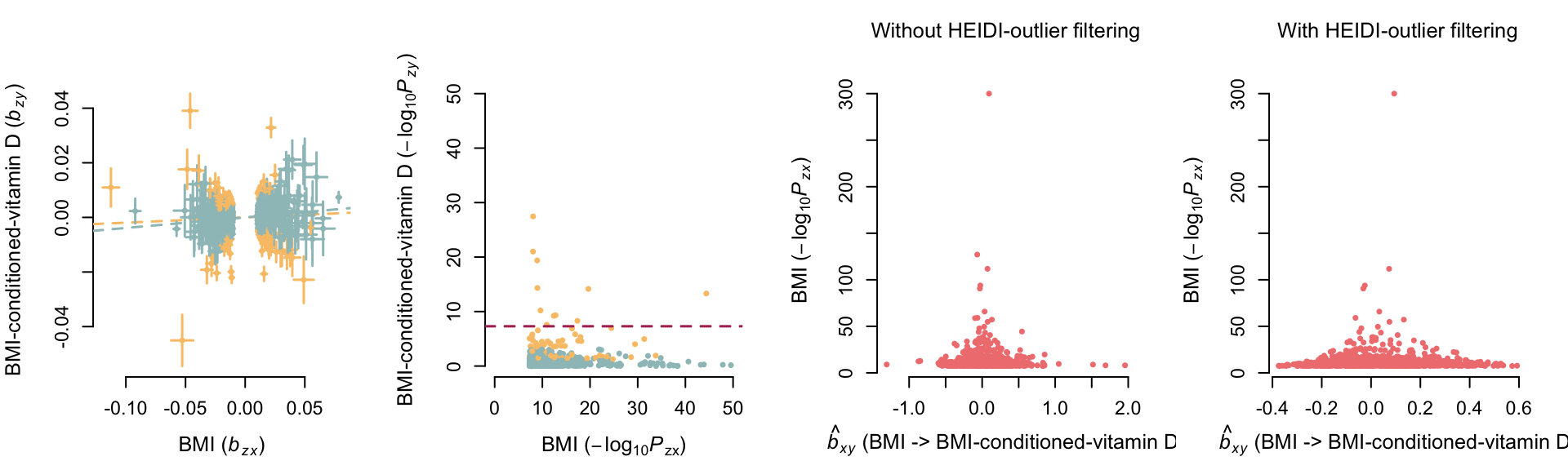
—– bxy obtained without
HEIDI-outlier method (i.e. including pleiotropic associations)
—– bxy obtained with
HEIDI-outlier method (i.e. after removing pleiotropic
associations)
Variants represented in yellow are
pleiotropic associations identified, and removed, with the HEIDI-outlier
method.
After mtCOJO the effect of BMI on vitamin D levels is greatly
attenuated.
2SMR
# Load and format 2SMR results
df=read.table("results/fastGWA/twosmr/ukbBMI.2smr", h=T, stringsAsFactors=F, sep="\t")
df$heidi=gsub(".*\\.","",df$exposure)
df$exposure=gsub("\\..*","",df$exposure)
df=df[,c("exposure","outcome","method","heidi","nsnp","b","se","pval")]
df=df[df$exposure=="ukbBMI",]

## Round results
  df$pval=format(df$pval, digits=3)
  cols=grep("se|b",names(df)); df[,cols]=apply(df[,cols], 2, function(x){round(x, 4)})

# Present table
datatable(df, rownames=FALSE,
          options=list(pageLength=5,
                       dom='frtipB',
                       buttons=c('csv', 'excel'),
                       scrollX=TRUE),
          caption="2SMR results for for BMi on 25OHD",
          extensions=c('Buttons','FixedColumns')) %>%
  formatStyle("pval","white-space"="nowrap")
Effect of vitamin D on BMI
GSMR before mtCOJO
# Get GSMR results beofre mtCOJO
gsmr_noHeidi=gsmr_noHeidi_bm
gsmr_newHeidi=gsmr_newHeidi_bm

# Define exposure and outcome
expo_str="Vitamin D"
outcome_str="BMI"


# ##############################################
# Plot GSMR results - Effect of vitamin D on BMI
# ##############################################
par(mfrow=c(1, 4))
par(mar=c(4.5, 4.5, 4, 2))

# Summary of results
tmp=as.data.frame(rbind(gsmr_noHeidi[[2]],gsmr_newHeidi[[2]]), stringsAsFactors=F)
tmp$Outcome=rep(c("Without HEIDI-outlier filtering","With HEIDI-outlier filtering"),each=2)
tmp=tmp[tmp$Exposure==expo_str,-1]
  # Add results from pleiotropic SNPs
  names(gsmr_vitDPleioSNPs_bm)[grep("nsnp",names(gsmr_vitDPleioSNPs_bm))]="n_snps"
  gsmr_vitDPleioSNPs_bm$Outcome="Pleiotropic SNPs"
  gsmr_vitDPleioSNPs_bm$Exposure=NULL
  tmp=rbind(tmp,gsmr_vitDPleioSNPs_bm)
names(tmp)[grep("Outcome",names(tmp))]=""
tmp=kable(tmp, row.names=F)
kable_styling(tmp, full_width=F, position = "left")| bxy | se | p | n_snps | |
|---|---|---|---|---|
| Without HEIDI-outlier filtering | -0.016529 | 0.00598459 | 0.00574623 | 277 |
| With HEIDI-outlier filtering | 0.00806448 | 0.00631405 | 0.201522 | 210 |
| Pleiotropic SNPs | -0.144461 | 0.0165637 | 2.74477e-18 | 67 |
# Define colors
effect_col=c("#9EC1C2","#FAC477")

# Identify pleiotropic SNPs
tmp=gsmr_noHeidi[[3]]
all_snps=tmp[tmp[,3]==1,1]
tmp=gsmr_newHeidi[[3]]
non_pleiotropic_snps=tmp[tmp[,3]==1,1]
pleiotropicSNP=factor(all_snps %in% non_pleiotropic_snps, levels=c("TRUE","FALSE"), labels=c("no","yes"))


# ---- Effect sizes in both GWAS
  # Define sumstats to plot
  resbuf = gsmr_snp_effect(gsmr_noHeidi, expo_str, outcome_str)
  bxy = resbuf$bxy
  bzx = resbuf$bzx; bzx_se = resbuf$bzx_se
  bzy = resbuf$bzy; bzy_se = resbuf$bzy_se
  tmp=gsmr_noHeidi[[2]]
  b=round(bxy,4)
  se=round(as.numeric(tmp[tmp[,1]==expo_str,4]), 4)
  p=format(as.numeric(tmp[tmp[,1]==expo_str,5]), digits=3)
  resbuf = gsmr_snp_effect(gsmr_newHeidi, expo_str, outcome_str)
  bxy2 = resbuf$bxy
  # Plot
    vals = c(bzx-bzx_se, bzx+bzx_se)
    xmin = min(vals); xmax = max(vals)
    vals = c(bzy-bzy_se, bzy+bzy_se)
    ymin = min(vals); ymax = max(vals)
    std = sd(vals)
    plot(bzx, bzy, pch=20, cex=0.8, bty="n", cex.axis=1.1, cex.lab=1.2,
         col=effect_col[pleiotropicSNP], xlim=c(xmin, xmax), ylim=c(ymin, ymax),
         xlab=substitute(paste(trait, " (", italic(b[zx]), ")", sep=""), list(trait=expo_str)),
         ylab=substitute(paste(trait, " (", italic(b[zy]), ")", sep=""), list(trait=outcome_str)))
    ## Regression line
    if(!is.na(bxy)) abline(0, bxy, lwd=1.5, lty=2, col=effect_col[2])
    if(!is.na(bxy)) abline(0, bxy2, lwd=1.5, lty=2, col=effect_col[1])
    ## Standard errors
    nsnps = length(bzx)
    for( i in 1:nsnps ) {
        # x axis
        xstart = bzx[i] - bzx_se[i]; xend = bzx[i] + bzx_se[i]
        ystart = bzy[i]; yend = bzy[i]
        segments(xstart, ystart, xend, yend, lwd=1.5, col=effect_col[pleiotropicSNP[i]])
        # y axis
        xstart = bzx[i]; xend = bzx[i]
        ystart = bzy[i] - bzy_se[i]; yend = bzy[i] + bzy_se[i]
        segments(xstart, ystart, xend, yend, lwd=1.5, col=effect_col[pleiotropicSNP[i]])
    }


# ---- P-values in both GWAS
plot_gsmr_pvalue(gsmr_noHeidi, expo_str, outcome_str, effect_col=effect_col[pleiotropicSNP])


# ---- P-value of exposure against effect size of
plot_bxy_distribution(gsmr_noHeidi, expo_str, outcome_str, effect_col="lightcoral")
mtext('Without HEIDI-outlier filtering', side=3, line=2, outer=F, cex=.8)
plot_bxy_distribution(gsmr_newHeidi, expo_str, outcome_str, effect_col="lightcoral")
mtext('With HEIDI-outlier filtering', side=3, line=2, outer=F, cex=.8)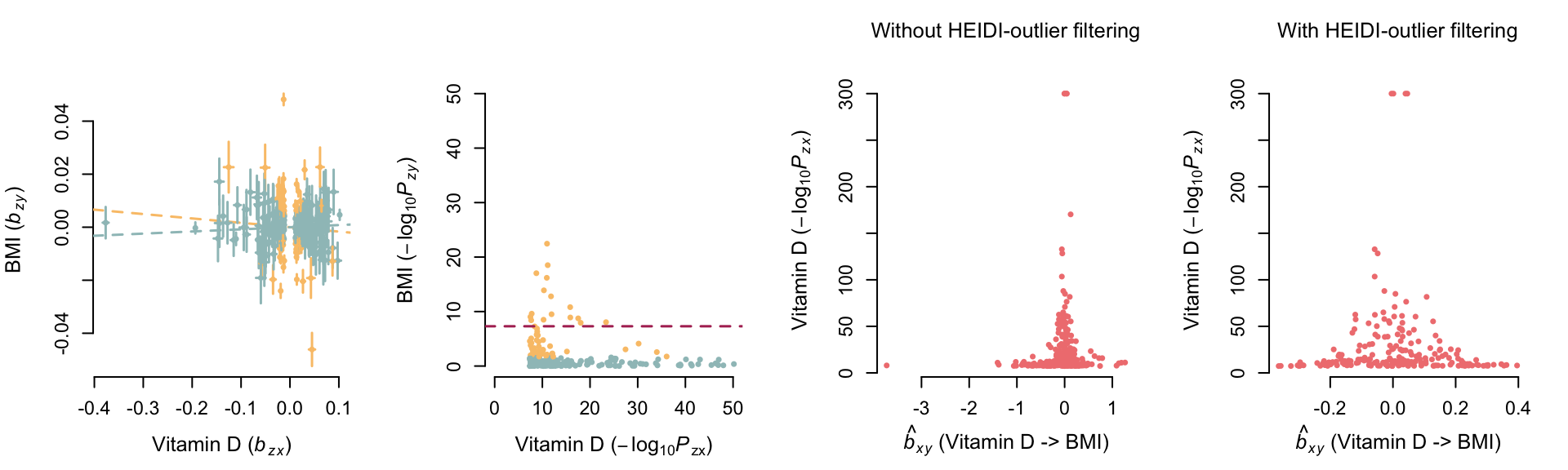
—– bxy obtained without
HEIDI-outlier method (i.e. including pleiotropic associations)
—– bxy obtained with
HEIDI-outlier method (i.e. after removing pleiotropic
associations)
Variants represented in yellow are
pleiotropic associations identified, and removed, with the HEIDI-outlier
method.
GSMR after mtCOJO
# Get GSMR results beofre mtCOJO
gsmr_noHeidi=gsmr_noHeidi_am
gsmr_newHeidi=gsmr_newHeidi_am

# Define exposure and outcome
expo_str="BMI-conditioned-vitamin D"
outcome_str="BMI"


# ##############################################
# Plot mtCOJO GSMR results - Effect of vitamin D on BMI
# ##############################################
par(mfrow=c(1, 4))
par(mar=c(4.5, 4.5, 4, 2))

# Summary of results
tmp=as.data.frame(rbind(gsmr_noHeidi[[2]],gsmr_newHeidi[[2]]))
tmp$Outcome=rep(c("Without HEIDI-outlier filtering","With HEIDI-outlier filtering"),each=2)
names(tmp)[grep("Outcome",names(tmp))]=""
tmp=kable(tmp[tmp$Exposure==expo_str,-1], row.names=F)
kable_styling(tmp, full_width=F, position = "left")| bxy | se | p | n_snps | |
|---|---|---|---|---|
| Without HEIDI-outlier filtering | 0.0214569 | 0.00594841 | 0.000309563 | 285 |
| With HEIDI-outlier filtering | 0.0143795 | 0.00624067 | 0.0212141 | 221 |
# Define colors
effect_col=c("#9EC1C2","#FAC477")

# Identify pleiotropic SNPs
tmp=gsmr_noHeidi[[3]]
all_snps=tmp[tmp[,3]==1,1]
tmp=gsmr_newHeidi[[3]]
non_pleiotropic_snps=tmp[tmp[,3]==1,1]
pleiotropicSNP=factor(all_snps %in% non_pleiotropic_snps, levels=c("TRUE","FALSE"), labels=c("no","yes"))


# ---- Effect sizes in both GWAS
  # Define sumstats to plot
  resbuf = gsmr_snp_effect(gsmr_noHeidi, expo_str, outcome_str)
  bxy = resbuf$bxy
  bzx = resbuf$bzx; bzx_se = resbuf$bzx_se
  bzy = resbuf$bzy; bzy_se = resbuf$bzy_se
  tmp=gsmr_noHeidi[[2]]
  b=round(bxy,4)
  se=round(as.numeric(tmp[tmp[,1]==expo_str,4]), 4)
  p=format(as.numeric(tmp[tmp[,1]==expo_str,5]), digits=3)
  resbuf = gsmr_snp_effect(gsmr_newHeidi, expo_str, outcome_str)
  bxy2 = resbuf$bxy
  # Plot
    vals = c(bzx-bzx_se, bzx+bzx_se)
    xmin = min(vals); xmax = max(vals)
    vals = c(bzy-bzy_se, bzy+bzy_se)
    ymin = min(vals); ymax = max(vals)
    std = sd(vals)
    plot(bzx, bzy, pch=20, cex=0.8, bty="n", cex.axis=1.1, cex.lab=1.2,
         col=effect_col[pleiotropicSNP], xlim=c(xmin, xmax), ylim=c(ymin, ymax),
         xlab=substitute(paste(trait, " (", italic(b[zx]), ")", sep=""), list(trait=expo_str)),
         ylab=substitute(paste(trait, " (", italic(b[zy]), ")", sep=""), list(trait=outcome_str)))
    ## Regression line
    if(!is.na(bxy)) abline(0, bxy, lwd=1.5, lty=2, col=effect_col[2])
    if(!is.na(bxy)) abline(0, bxy2, lwd=1.5, lty=2, col=effect_col[1])
    ## Standard errors
    nsnps = length(bzx)
    for( i in 1:nsnps ) {
        # x axis
        xstart = bzx[i] - bzx_se[i]; xend = bzx[i] + bzx_se[i]
        ystart = bzy[i]; yend = bzy[i]
        segments(xstart, ystart, xend, yend, lwd=1.5, col=effect_col[pleiotropicSNP[i]])
        # y axis
        xstart = bzx[i]; xend = bzx[i]
        ystart = bzy[i] - bzy_se[i]; yend = bzy[i] + bzy_se[i]
        segments(xstart, ystart, xend, yend, lwd=1.5, col=effect_col[pleiotropicSNP[i]])
    }


# ---- P-values in both GWAS
plot_gsmr_pvalue(gsmr_noHeidi, expo_str, outcome_str, effect_col=effect_col[pleiotropicSNP])


# ---- P-value of exposure against effect size of
plot_bxy_distribution(gsmr_noHeidi, expo_str, outcome_str, effect_col="lightcoral")
mtext('Without HEIDI-outlier filtering', side=3, line=2, outer=F, cex=.8)
plot_bxy_distribution(gsmr_newHeidi, expo_str, outcome_str, effect_col="lightcoral")
mtext('With HEIDI-outlier filtering', side=3, line=2, outer=F, cex=.8)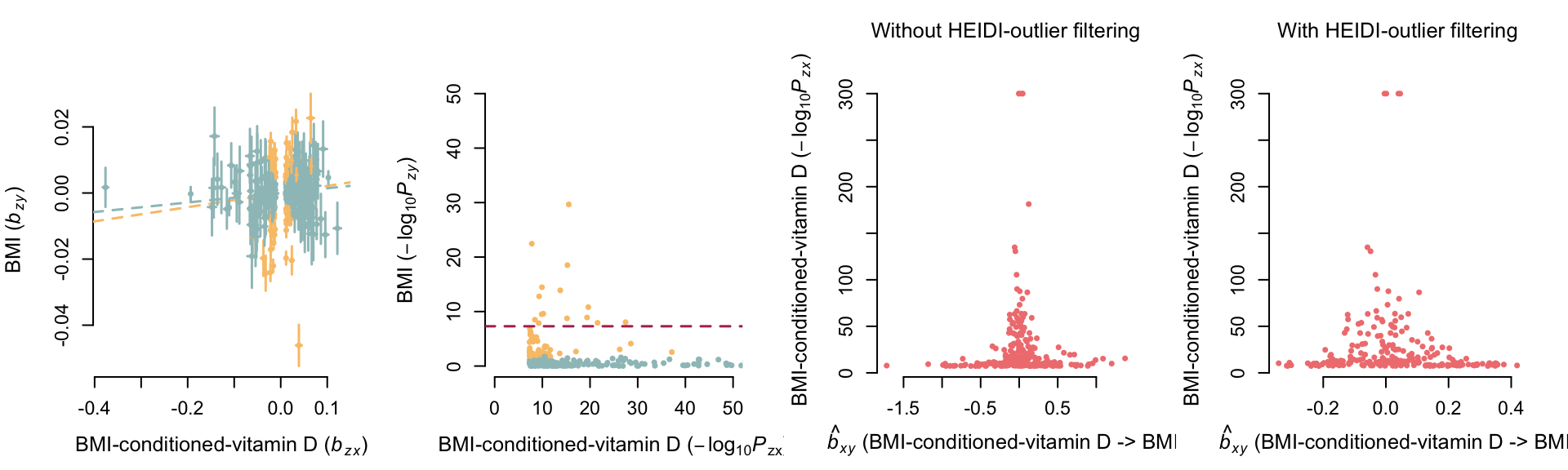
—– bxy obtained without
HEIDI-outlier method (i.e. including pleiotropic associations)
—– bxy obtained with
HEIDI-outlier method (i.e. after removing pleiotropic
associations)
Variants represented in yellow are
pleiotropic associations identified, and removed, with the HEIDI-outlier
method.
2SMR
# Load and format 2SMR results
df=read.table("results/fastGWA/twosmr/ukbBMI.2smr", h=T, stringsAsFactors=F, sep="\t")
df$heidi=gsub(".*\\.","",df$exposure)
df$exposure=gsub("\\..*","",df$exposure)
df=df[,c("exposure","outcome","method","heidi","nsnp","b","se","pval")]
df=df[df$exposure=="vitD",]

## Round results
  df$pval=format(df$pval, digits=3)
  cols=grep("se|b",names(df)); df[,cols]=apply(df[,cols], 2, function(x){round(x, 4)})

# Present table
datatable(df, rownames=FALSE,
          options=list(pageLength=5,
                       dom='frtipB',
                       buttons=c('csv', 'excel'),
                       scrollX=TRUE),
          caption="2SMR results for for BMi on 25OHD",
          extensions=c('Buttons','FixedColumns')) %>%
  formatStyle("pval","white-space"="nowrap")
25OHD conditioned on BMI (mtCOJO)
# ########################
# Summarise mtCOJO results
# ########################

# mtCOJO (vitamin D condition on BMI)
#mtcojo=read.table("results/fastGWA/mtcojo.vitD_fastGWA_condition_on_ukbBMI.mtcojo.cma",h=T,stringsAsFactors = F)
#mtcojo=merge(mtcojo,vitD[,c("SNP","CHR","BP")])
#saveRDS(mtcojo, file="results/fastGWA/mtcojo.vitD_fastGWA_condition_on_ukbBMI.mtcojo.RDS")
mtcojo=readRDS("results/fastGWA/mtcojo.vitD_fastGWA_condition_on_ukbBMI.mtcojo.RDS")
cojo_vitD_BMIcond=read.table("results/fastGWA/mtcojo.vitD_fastGWA_condition_on_ukbBMI.cojo", h=T, stringsAsFactors=F)
Summary of results
After conditioning the vitamin D GWAS results on BMI (with mtCOJO), we have:
- 7250403 variants tested – none in the X chromosome, as the BMI GWAS did not have summary statistics on the X chromosome
- 16012 genome-wide significant (GWS;
P<5x10⁻⁸) hits
- 155 independent variants (determined with
COJO)
- 147 independent variants (determined with COJO)
that were GWS in the original GWAS
# ################################################
# Present list of independent associations (identified with COJO)
# ################################################
indep = cojo_vitD_BMIcond %>% arrange(Chr, bp)

# Format table
indep=indep[,c("Chr","SNP","bp","refA","freq","b","se","p","n","freq_geno","bJ","bJ_se","pJ")]
indep$p=format(indep$p, digits=3)
indep$pJ=format(indep$pJ, digits=3)
  options(warn=-1)
indep=indep %>% mutate_at(vars(se, bJ_se, b, bJ), funs(round(., 4)))
  options(warn=0)
indep=indep %>% mutate_at(vars(freq, freq_geno), funs(round(., 2)))
## Warning: `funs()` was deprecated in dplyr 0.8.0.
## ℹ Please use a list of either functions or lambdas:
##
## # Simple named list: list(mean = mean, median = median)
##
## # Auto named with `tibble::lst()`: tibble::lst(mean, median)
##
## # Using lambdas list(~ mean(., trim = .2), ~ median(., na.rm = TRUE))# Present table
datatable(indep,
rownames=FALSE,
extensions=c('Buttons','FixedColumns'),
options=list(pageLength=5,
dom='frtipB',
buttons=c('csv', 'excel'),
scrollX=TRUE),
caption="List of independent associations") %>%
formatStyle("p","white-space"="nowrap") %>%
formatStyle("pJ","white-space"="nowrap")Columns are: Chr, chromosome; SNP, SNP rs ID; bp, physical position; refA, the effect allele; type, type of QTL; freq, frequency of the effect allele in the original data; b, se and p, effect size, standard error and p-value from the original GWAS; n, estimated effective sample size; freq_geno, frequency of the effect allele in the reference sample; bJ, bJ_se and pJ, effect size, standard error and p-value from a joint analysis of all the selected SNPs.