Vitamin D GWAS

# Libraries
library(ggplot2)
library(dplyr)
library(ggrepel)
library(DT)
library(qqman)
library(knitr)
library(kableExtra)

---

We ran a classical genome-wide association (GWA) analysis with fastGWA. The aim was to test the association between alleles and the mean of a phenotype and identify quantitative trait loci (QLT), i.e. variants that are associated with variability in the trait.

Below we describe our analyses and present the results.

---

Methods

GWAS

This analysis was performed with fastGWA using variants with MAF>0.01. Given our sample size (N=417580), this is equivalent to restricting to SNPs seen at least 8351.6 times.

Chromosome X and its pseudo-autosomal region were analysed separately in males and females and were subsequently meta-analysed with METAL, using the inverse-variance based method. Only variants with MAF>0.01 in females were analysed.

The following files were used to run the analysis:

• Phenotype file: This file includes one line per individual and a column with the phenotype. The phenotype was obtained after (1) restricting to individuals of European ancestry, and (2) applying a rank-based inverse-normal transformation. In total 417580 individuals of European ancestry were analysed.
• Genotype file: We used genotype files that were restricted to individuals of European ancestry and included 44741804 autossomal variants + 260713 variants in chromosome X (including the pseudo-autosomal region). Variants had (1) MAC > 5, (2) INFO > 0.3, and (3) genotype missingness > 0.05. In addition, variants with missingness < 0.05, pHWE < 1x10^-5, and MAC > 5 in the subset of unrelated European individuals were excluded.
• Sparse GRM: For this analysis we used a sparse GRM that was calculated using HapMap3 SNPs from individuals of European ancestry.
  
• Covariates files: This file includes one column per covariate to fit in the model. Covariates included were: age, sex, genotyping batch, UKB assessment centre, assessment month, information on whether vitamin supplements were ever taken, and the first 40 PCs. For more detail see the covariates section of the Pheno page.

To run the analysis faster, associations were performed by chromosome and ran in parallel. qsubshcom was used to submit the parallel jobs (array).

# Directories
genoDir=$medici/v3EUR_impQC


# #########################################
# Prepare files for analysis
# #########################################

# ------ Get sparse GRM 
## Run from delta
cp $longda/UKB_geno/UKB_sparse_GRM/UKB_HM3_m01_sp.grm* $WD/input


# ------ Get list of SNPs to include in the analysis
# Extract common (MAF>0.01) variants
geno=$medici/v3EUR_impQC/ukbEUR_imp_chr{TASK_ID}_v3_impQC
filters=maf0.01
genoDir=$WD/input/UKB_v3EUR_impQC
snpList=$genoDir/UKB_EUR_impQC_$filters
cd $genoDir
tmp_command="plink --bfile $geno \
                   --write-snplist \
                   --maf 0.01 \
                   --out ${snpList}_chr{TASK_ID}"
qsubshcom "$tmp_command" 1 10G commonVariants 3:00:00 "-array=1-22"
cat ${snpList}_chr*.snplist > $snpList.snplist
rm ${snpList}_chr*




# ------ Make mbfile with all individual-level data files to include in the analysis
tmpDir=$WD/results/fastGWA/tmpDir
echo $genoDir/ukbEUR_imp_chr1_v3_impQC > $tmpDir/UKB_v3EUR_impQC.files
for i in `seq 2 22`; do echo $genoDir/ukbEUR_imp_chr${i}_v3_impQC >> $tmpDir/UKB_v3EUR_impQC.files; done




# #########################################
# Run GWAS with fastGWA - autosomes
# #########################################

# Set directories
results=$WD/results/fastGWA
tmpDir=$results/tmpDir

# Files/settings to use
prefix=vitD_fastGWA
#prefix=vitD_BMIcov_fastGWA
geno=$tmpDir/UKB_v3EUR_impQC.files
pheno=$WD/input/mlm_pheno
grm=$WD/input/UKB_HM3_m01_sp
quantCovars=$WD/input/quantitativeCovariates
#quantCovars=$WD/input/quantitativeCovariates_bmi
catgCovars=$WD/input/categoricalCovariates
snps2include=$WD/input/UKB_v3EUR_impQC/UKB_EUR_impQC_maf0.01.snplist
output=$tmpDir/$prefix

# Run GWAS
cd $results
gcta=$bin/gcta/gcta_1.92.3beta3
tmp_command="$gcta --mbfile $geno \
                   --fastGWA-lmm \
                   --pheno $pheno \
                   --grm-sparse  $grm \
                   --qcovar $quantCovars\
                   --covar $catgCovars \
                   --covar-maxlevel 110 \
                   --extract $snps2include \
                   --threads 16 \
                   --out $output"
qsubshcom "$tmp_command" 16 10G $prefix 24:00:00 ""

# Compress results
gzip -c $output.fastGWA > $results/$prefix.gz


# Convert GWAS sumstats to .ma format (for COJO)
echo "SNP A1 A2 freq b se p n" > $results/maFormat/$prefix.ma
awk '{print $2,$4,$5,$7,$8,$9,$10,$6}' $tmpDir/$prefix.fastGWA | sed 1d >> $results/maFormat/$prefix.ma



# #########################################
# Run GWAS with fastGWA - X chromosome
# #########################################

# Set directories
results=$WD/results/fastGWA
tmpDir=$results/tmpDir

# Files/settings to use
pheno=$WD/input/mlm_pheno
grm=$WD/input/UKB_HM3_m01_sp
quantCovars=$WD/input/quantitativeCovariates
#quantCovars=$WD/input/quantitativeCovariates_bmi
catgCovars=$WD/input/categoricalCovariates_noSex

# ---- Run GWAS separately for males and females
cd $results
for sex in FEMALE MALE
do
  # Run X chromosome pseudo-autosomal region (chr XY) as well
  for region in X XY
  do
    prefix=vitD_fastGWA_chr$region.$sex
    #prefix=vitD_BMIcov_fastGWA_chr$region.$sex
    geno=$medici/v3EUR_chrX/ukbEURv3_${region}_maf0.1_$sex
    output=$tmpDir/$prefix
  
    gcta=$bin/gcta/gcta_1.92.3beta3
    tmp_command="$gcta --bfile $geno \
                       --fastGWA-lmm \
                       --pheno $pheno \
                       --grm-sparse  $grm \
                       --qcovar $quantCovars\
                       --covar $catgCovars \
                       --covar-maxlevel 110 \
                       --threads 16 \
                       --out $output"
    qsubshcom "$tmp_command" 16 30G $prefix 6:00:00 ""
  done
done


# #########################################
# Meta-analyse results from males and females for X and XY
# #########################################

cd $WD/results/fastGWA/tmpDir
metal=$bin/metal/metal
$metal

# === CHROMOSOME X ================================================
CLEAR
SCHEME STDERR
AVERAGEFREQ ON

# Describe and process results for X chromosome
MARKER SNP
ALLELE A1 A2
EFFECT BETA
PVALUE P
WEIGHT N
STDERR SE
FREQLABEL AF1

PROCESS $WD/results/fastGWA/tmpDir/vitD_fastGWA_chrX.FEMALE.fastGWA
PROCESS $WD/results/fastGWA/tmpDir/vitD_fastGWA_chrX.MALE.fastGWA
#PROCESS $WD/results/fastGWA/tmpDir/vitD_BMIcov_fastGWA_chrX.FEMALE.fastGWA
#PROCESS $WD/results/fastGWA/tmpDir/vitD_BMIcov_fastGWA_chrX.MALE.fastGWA

# Run meta-analysis
OUTFILE $WD/results/fastGWA/tmpDir/vitD_fastGWA_chrX .TBL
#OUTFILE $WD/results/fastGWA/tmpDir/vitD_BMIcov_fastGWA_chrX .TBL

ANALYZE

# === CHROMOSOME XY (X chromosome pseudo-autosomal region) ========
CLEAR
SCHEME STDERR
AVERAGEFREQ ON

# Describe and process results for XY chromosome
MARKER SNP
ALLELE A1 A2
EFFECT BETA
PVALUE P 
WEIGHT N
STDERR SE
FREQLABEL AF1

PROCESS $WD/results/fastGWA/tmpDir/vitD_fastGWA_chrXY.FEMALE.fastGWA
PROCESS $WD/results/fastGWA/tmpDir/vitD_fastGWA_chrXY.MALE.fastGWA
#PROCESS $WD/results/fastGWA/tmpDir/vitD_BMIcov_fastGWA_chrXY.FEMALE.fastGWA
#PROCESS $WD/results/fastGWA/tmpDir/vitD_BMIcov_fastGWA_chrXY.MALE.fastGWA

# Run meta-analysis
OUTFILE $WD/results/fastGWA/tmpDir/vitD_fastGWA_chrXY .TBL
#OUTFILE $WD/results/fastGWA/tmpDir/vitD_BMIcov_fastGWA_chrXY .TBL
ANALYZE


# #########################################
# Format meta-analysed results and merge with autossomes
# Generate .ma format files for COJO
# #########################################

setwd("results/fastGWA")

prefix="vitD_fastGWA"
#prefix="vitD_BMIcov_fastGWA"

# Read X meta-analyses results + GWAS results for autosomes
xmeta=read.table(paste0("tmpDir/",prefix,"_chrX1.TBL"),h=T,stringsAsFactors=F)
xymeta=read.table(paste0("tmpDir/",prefix,"_chrXY1.TBL"),h=T,stringsAsFactors=F)
autosomes=read.table(paste0("tmpDir/",prefix,".fastGWA"), h=T,stringsAsFactors=F)
names(xmeta)=c("SNP","A1","A2","AF1","AF1_SE","BETA","SE","P","direction")
names(xymeta)=c("SNP","A1","A2","AF1","AF1_SE","BETA","SE","P","direction")

# Get chrX details (BP, allele freq, and N) from female and male GWAS
xfemale=read.table(paste0("tmpDir/",prefix,"_chrX.FEMALE.fastGWA"), h=T,stringsAsFactors=F)
xmale=read.table(paste0("tmpDir/",prefix,"_chrX.MALE.fastGWA"), h=T,stringsAsFactors=F)
  ## Get all results in the same order
  xmeta=xmeta[match(xfemale$SNP,xmeta$SNP),]
  xmale=xmale[match(xfemale$SNP,xmale$SNP),]
  ## Add BP
  xmeta$POS=xfemale$POS
  # Add N
  xmeta$N=xfemale$N+xmale$N
  # Change alleles to capital letters
  xmeta$A1=toupper(xmeta$A1)
  xmeta$A2=toupper(xmeta$A2)
  # Define chromosome
  xmeta$CHR=23
  
# Get chrXY details (BP, allele freq, and N) from female and male GWAS
xyfemale=read.table("tmpDir/vitD_fastGWA_chrXY.FEMALE.fastGWA", h=T,stringsAsFactors=F)
xymale=read.table("tmpDir/vitD_fastGWA_chrXY.MALE.fastGWA", h=T,stringsAsFactors=F)
  ## Get all results in the same order
  xymeta=xymeta[match(xyfemale$SNP,xymeta$SNP),]
  xymale=xymale[match(xyfemale$SNP,xymale$SNP),]
  ## Add BP
  xymeta$POS=xyfemale$POS
  ## Add N
  xymeta$N=xyfemale$N+xymale$N
  # Define chromosome
  xymeta$CHR=25
  # Change alleles to capital letters
  xymeta$A1=toupper(xymeta$A1)
  xymeta$A2=toupper(xymeta$A2)

# fastGWA format
# CHR SNP POS A1 A2 N AF1 BETA SE P
  xmeta_fastgwa=xmeta[,c("CHR","SNP","POS","A1","A2","N","AF1","BETA","SE","P")]
  xymeta_fastgwa=xymeta[,c("CHR","SNP","POS","A1","A2","N","AF1","BETA","SE","P")]
  ## Merge X + XY + autosomes
  allChr=rbind(autosomes, xmeta_fastgwa, xymeta_fastgwa)

# COJO (.ma) format
# SNP A1 A2 freq b se p n
 ## CHR X
 xmeta_ma=xmeta[,c("SNP","A1","A2","AF1","BETA","SE","P","N")]
 names(xmeta_ma)=c("SNP","A1","A2","freq","b","se","p","n")
  ## CHR XY
 xymeta_ma=xymeta[,c("SNP","A1","A2","AF1","BETA","SE","P","N")]
 names(xymeta_ma)=c("SNP","A1","A2","freq","b","se","p","n")
  

# Save new file formats
  ## All chromosomes
  write.table(allChr, file=gzfile(paste0(prefix,"_withX.gz")), quote=F, row.names=F)
  ## X and XY in fastGWA format (for clumping)
  write.table(xmeta_fastgwa, file=gzfile(paste0("tmpDir/",prefix,"_chrX.gz")), quote=F, row.names=F)
  write.table(xymeta_fastgwa, file=gzfile(paste0("tmpDir/",prefix,"_chrXY.gz")), quote=F, row.names=F)
  ## X and XY in .ma format (for COJO)
  write.table(xmeta_ma, paste0("maFormat/",prefix,"_chrX.ma"), quote=F, row.names=F)
  write.table(xymeta_ma, paste0("maFormat/",prefix,"_chrXY.ma"), quote=F, row.names=F)


# #########################################
# Make .ma file with all chr (including X)
# #########################################

prefix=vitD_fastGWA
#prefix=vitD_BMIcov_fastGWA
results=$WD/results/fastGWA/maFormat

cp $results/$prefix.ma $results/${prefix}_withX.ma 
sed 1d $results/${prefix}_chrX.ma >> $results/${prefix}_withX.ma 
sed 1d $results/${prefix}_chrXY.ma >> $results/${prefix}_withX.ma 

Clump

Results were then clumped with plink 1.9. The following options were used in this analysis:

• –bfile - v3EUR_impQC samples were used as reference for the autosomes. v3EUR_impQC female samples were used as reference for the X chromosome and the X chromosome pseudo-autossomal region
• –clump-p1 = 5x10^-8 - max P-value for index variants to start a clump
• –clump-p2 = 0.01 (default) - max P-value for variants in a clump to be listed in column SP2
• –clump-r2 = 0.01 - minimum r2 with index variant for a site to be included in that clump
• –clump-kb = 10,000 - maximum distance from index SNP for a site to be included in that clump

# There are duplicated SNPs in the v3EUR_impQC files. This causes an error when running clumping using them as LD reference. 
# Generate a file with their rs IDs and exclude them from analysis when clumping
for i in `seq 1 22`
do 
  echo $i
  awk '{print $2}' $medici/v3EUR_impQC/ukbEUR_imp_chr${i}_v3_impQC.bim | sort | uniq -d >> $WD/input/UKB_v3EUR_impQC/UKB_EUR_impQC_duplicated_rsIDs
done


# #########################################
# Clump GWAS results - autossomes
# #########################################

# Directories
results=$WD/results/fastGWA
tmpDir=$results/tmpDir

# Files/settings to use
prefix=vitD_fastGWA
#prefix=vitD_BMIcov_fastGWA
ref=$medici/v3EUR_impQC/ukbEUR_imp_chr{TASK_ID}_v3_impQC
inFile=$tmpDir/$prefix.fastGWA
outFile=$tmpDir/${prefix}_chr{TASK_ID}
snps2exclude=$WD/input/UKB_v3EUR_impQC/UKB_EUR_impQC_duplicated_rsIDs
window=10000
jobName=$prefix.clump


# Run clumping
cd $results
plink=$bin/plink/plink-1.9/plink
tmp_command="$plink --bfile $ref \
                    --exclude $snps2exclude \
                    --clump $inFile \
                    --clump-p1 5e-8 \
                    --clump-r2 0.01 \
                    --clump-kb $window \
                    --clump-field "P" \
                    --out $outFile"          
qsubshcom "$tmp_command" 1 30G $jobName 24:00:00 "-array=1-22"



# #########################################
# Clump GWAS results - chromosome X
# #########################################

# Directories
results=$WD/results/fastGWA
tmpDir=$results/tmpDir

# Run clumping
cd $results
for chr in X XY
do 
  # Files/settings to use
  prefix=vitD_fastGWA_chr$chr
  #prefix=vitD_BMIcov_fastGWA_chr$chr
  ref=$medici/v3EUR_chrX/ukbEURv3_${chr}_maf0.1_FEMALE
  inFile=$tmpDir/$prefix.gz
  outFile=$tmpDir/$prefix
  plink=$bin/plink/plink-1.9/plink
  tmp_command="$plink --bfile $ref \
                      --clump $inFile \
                      --clump-p1 5e-8 \
                      --clump-r2 0.01 \
                      --clump-kb 10000 \
                      --clump-field "P" \
                      --out $outFile"          
  qsubshcom "$tmp_command" 1 10G $prefix.clump 10:00:00 ""
  echo $prefix.clump
done

# #########################################
# Merge clumped results once all chr finished running
# #########################################
cat $tmpDir/${prefix}_chr*clumped | grep "CHR" | head -1 > $results/${prefix}_withX.clumped
cat $tmpDir/${prefix}_chr*clumped | grep -v "CHR" |sed '/^$/d'  >> $results/${prefix}_withX.clumped

COJO

COJO – a summary-statistics-based method implemented in GCTA – is an approach to identify independent associations. It starts with the most associated SNP, then, conditioning on that SNP, it finds the second most associated SNP. Then, conditioning on both those SNPs, it finds the third most associated SNP, and so on.

The following options were used in this analysis:

• –bfile: For the autosomes, we used a random subset of 20,000 unrelated individuals of European ancestry from the UKB as LD reference. For the X chromosome, we used female samples as LD reference.
• –cojo-slct: Performs a step-wise model selection of independently associated SNPs
• –cojo-p 5e-8 (default): P-value to declare a genome-wide significant hit
• –cojo-wind 10,000 (default): Distance (in KB) from which SNPs are considered in linkage equilibrium
• –cojo-collinear 0.9 (default): maximum r2 to be considered an independent SNP, i.e. SNPs with r2>0.9 will not be considered further
• –diff-freq 0.2 (default): maximum allele difference between the GWAS and the LD reference sample
• extract: Restrict analysis to SNPs with MAF>0.01

# ########################
# Prepare files to run COJO
# ########################

# --- Extract a random set of 20K unrelated Europeans to use as LD reference for the autosomes
#     In addition, keep only the variants in the vitamin D GWAS to speed up GSMR analysis
  # Extract SNPs in fastGWA results
  prefix=vitD_fastGWA
  results=$WD/results/fastGWA

  random20k_dir=$WD/input/UKB_v3EURu_impQC/random20K
  awk 'NR>1{print $2}' $tmpDir/$prefix.fastGWA |  > $random20k_dir/$prefix.snpList
  
  # Extract data
  ld_ref=$medici/v3EURu_impQC/ukbEURu_imp_chr{TASK_ID}_v3_impQC
  ids2keep=$medici/v3Samples/ukbEURu_v3_all_20K.fam
  snps2keep=$WD/input/UKB_v3EURu_impQC/random20K/$prefix.snpList
  output=$random20k_dir/ukbEURu_imp_chr{TASK_ID}_v3_impQC_random20k_maf0.01

  cd $random20k_dir
  plink=$bin/plink/plink-1.9/plink
  tmp_command="$plink --bfile $ld_ref  \
                      --keep $ids2keep \
                      --extract $snps2keep  \
                      --make-bed \
                      --out $output"
  qsubshcom "$tmp_command" 1 10G ukbEURu_v3_impQC_random20k_maf0.01 24:00:00 "-array=1-22"


# #########################################
# Run COJO on GWAS results - autosomes
# #########################################

gcta=$bin/gcta/gcta_1.92.3beta3

# Common settings
prefix=vitD_fastGWA
#prefix=vitD_BMIcov_fastGWA
results=$WD/results/fastGWA
tmpDir=$results/tmpDir
random20k_dir=$WD/input/UKB_v3EURu_impQC/random20K
ldRef=$random20k_dir/ukbEURu_imp_chr{TASK_ID}_v3_impQC_random20k_maf0.01
filters=maf0.01
window=10000
inFile=$results/maFormat/$prefix.ma
snps2include=$WD/input/UKB_v3EUR_impQC/UKB_EUR_impQC_$filters.snplist
outFile=$tmpDir/${prefix}_${filters}_chr{TASK_ID}
jobName=$prefix.COJO
  
# Run COJO
cd $results
tmp_command="$gcta --bfile $ldRef \
                   --cojo-slct \
                   --cojo-file $inFile \
                   --cojo-wind $window \
                   --extract $snps2include \
                   --out $outFile"
                             
qsubshcom "$tmp_command" 1 100G $jobName 24:00:00 "-array=1-22 $account"


# #########################################
# Run COJO on GWAS results - X chromosome
# #########################################

# Common settings
prefix=vitD_fastGWA
#prefix=vitD_BMIcov_fastGWA
results=$WD/results/fastGWA
tmpDir=$results/tmpDir
filters=maf0.01

# Run COJO
cd $results
gcta=$bin/gcta/gcta_1.92.3beta3
for chr in X XY
do
  ref=$medici/v3EUR_chrX/ukbEURv3_${chr}_maf0.1_FEMALE
  inFile=$results/maFormat/${prefix}_chr$chr.ma
  outFile=$tmpDir/${prefix}_${filters}_chr$chr
  tmp_command="$gcta --bfile $ref \
                   --cojo-slct \
                   --cojo-file $inFile \
                   --maf 0.01 \
                   --out $outFile"
                             
  qsubshcom "$tmp_command" 1 30G ${prefix}_chr$chr.COJO 24:00:00 "$account"
done

# #########################################
# Merge COJO results once all chr finished running
# #########################################
cat $tmpDir/${prefix}_${filters}*.jma.cojo | grep "Chr" | uniq > $results/${prefix}_${filters}_withX.cojo
cat $tmpDir/${prefix}_${filters}_chr*.jma.cojo | grep -v "Chr" |sed '/^$/d'  >> $results/${prefix}_${filters}_withX.cojo

To assess the number of significant associations that were independent from previously reported variants, we performed an association analysis conditional on the 6 following SNPs:

• rs2282679
• rs10741657
• rs12785878
• rs10745742
• rs8018720
• rs6013897

Specifically, we used the --cojo-cond option implemented in GCTA for this analysis.

# ------ Condition GWAS results on known variants
# Delta settings
gcta=$bin/gcta/gcta_1.92.3beta3

# Common settings
prefix=vitD_fastGWA
results=$WD/results/fastGWA
tmpDir=$results/tmpDir
random20k_dir=$WD/input/UKB_v3EURu_impQC/random20K
ldRef=$random20k_dir/ukbEURu_imp_chr{TASK_ID}_v3_impQC_random20k_maf0.01
filters=maf0.01
inFile=$results/maFormat/$prefix.ma
snps2include=$WD/input/UKB_v3EUR_impQC/UKB_EUR_impQC_$filters.snplist
outFile=$tmpDir/${prefix}_${filters}_conditionOnKnownLoci_chr{TASK_ID}
knownLoci=$WD/input/vitD_knownLoci.txt

# Generate list of known variants
loci2conditionOn=$tmpDir/knownLoci
awk 'NR>1 {print $1}' $knownLoci > $loci2conditionOn

# Condition GWAS results on known variants
cd $results
tmp_command="$gcta --bfile $ldRef \
                   --cojo-file $inFile \
                   --extract $snps2include \
                   --cojo-cond $loci2conditionOn \
                   --out $outFile"
                             
qsubshcom "$tmp_command" 1 100G $prefix.COJO.knownLoci 24:00:00 "-array=1-22 $account"




# ------ Create file with all results after conditioning on known variants
  ## Run this step in R
  knownLoci=read.table("input/vitD_knownLoci.txt", h=T, stringsAsFactors=F, sep="\t")
  
  # Load all results and 
  gwas=read.table("results/fastGWA/vitD_fastGWA_withX.gz", h=T, stringsAsFactors=F)
  
  # Keep SNP information from CHR that have been condition on known SNPs and remove results (we'll use the conditioned ones) 
  knownLoci_SNPinfo=gwas[gwas$CHR %in% knownLoci$CHR,c("SNP","A1","A2")]
  gwas=gwas[!gwas$CHR %in% knownLoci$CHR,]
  
  # Add conditioned results
  for(chr in unique(knownLoci$CHR))
  {
    print(chr)
    tmp=read.table(paste0("results/fastGWA/tmpDir/vitD_fastGWA_maf0.01_conditionOnKnownLoci_chr",chr,".cma.cojo"), h=T, stringsAsFactors=F)
    # Add information not provided in COJO output (A2)
    tmp=merge(tmp,knownLoci_SNPinfo, all.x=T)
    if(!identical(tmp$A1,tmp$refA)){print("Check alleles")}
    # Merge with unconditioned results
    tmp=tmp[,c("Chr","SNP","bp","A1","A2","n","freq","bC","bC_se","pC")]
    names(tmp)=c("CHR","SNP","POS","A1","A2","N","AF1","BETA","SE","P")
    gwas=rbind(gwas,tmp)
  }
  
  # Save conditioned results
  write.table(gwas, file=gzfile("results/fastGWA/vitD_fastGWA_withX_conditionOnKnownLoci.gz"), quote=F, row.names=F)
  
  # Convert to .ma format (to run COJO) and save
  ## SNP A1 A2 freq b se p n
  maFormat=gwas[,c("SNP","A1","A2","AF1","BETA","SE","P","N")]
  names(maFormat)=c("SNP","A1","A2","freq","b","se","p","n")
  write.table(maFormat, "results/fastGWA/maFormat/vitD_fastGWA_withX_conditionOnKnownLoci.ma", quote=F, row.names=F)
  
  

# ------ Run COJO on conditioned results

# Delta settings
gcta=$bin/gcta/gcta_1.92.3beta3

# Common settings
prefix=vitD_fastGWA_withX_conditionOnKnownLoci
results=$WD/results/fastGWA
tmpDir=$results/tmpDir
random20k_dir=$WD/input/UKB_v3EURu_impQC/random20K
ldRef=$random20k_dir/ukbEURu_imp_chr{TASK_ID}_v3_impQC_random20k_maf0.01
filters=maf0.01
inFile=$results/maFormat/$prefix.ma
snps2include=$WD/input/UKB_v3EUR_impQC/UKB_EUR_impQC_$filters.snplist
outFile=$tmpDir/${prefix}_${filters}_chr{TASK_ID}
knownLoci=$WD/input/vitD_knownLoci.txt

cd $results
tmp_command="$gcta --bfile $ldRef \
                   --cojo-slct \
                   --cojo-file $inFile \
                   --extract $snps2include \
                   --out $outFile"
qsubshcom "$tmp_command" 1 30G $prefix.COJO 24:00:00 "-array=1-22 $account"



cat $tmpDir/${prefix}_${filters}*.jma.cojo | grep "Chr" | uniq > $results/${prefix}_${filters}.cojo
cat $tmpDir/${prefix}_${filters}_chr*.jma.cojo | grep -v "Chr" |sed '/^$/d'  >> $results/${prefix}_${filters}.cojo

LDSC

To run LDSC, we restricted the GWAS summary statistics to variants found in w_hm3.noMHC.snplist (downloaded from LDHub). This is a list of HapMap3 SNPs and excludes SNPs in the MHC region. Note that this does not include variants on the X chromosome.

module load ldsc
prefix=vitD_fastGWA
#prefix=vitD_BMIcov_fastGWA

# Directories
results=$WD/results/fastGWA
tmpDir=$results/tmpDir
ldscDir=$bin/ldsc

# Format GWAS results
awk '{print $1,$2,$3,$5,$8,$7}' $results/maFormat/$prefix.ma > $tmpDir/$prefix.ldHubFormat

# Restrict to common SNPs
sed 1q $tmpDir/$prefix.ldHubFormat > $results/ldscFormat/$prefix.ldHubFormat
awk 'NR==FNR{a[$1];next} ($1 in a)' $WD/input/UKB_v3EURu_impQC/UKB_EURu_impQC_maf0.01.snplist <(awk 'NR==FNR{a[$1];next} ($1 in a)' $WD/input/w_hm3.noMHC.snplist $tmpDir/$prefix.ldHubFormat) >> $results/ldscFormat/$prefix.ldHubFormat

# Munge sumstats (process sumstats and restrict to HapMap3 SNPs)
cd $results/ldscFormat/
munge_sumstats.py --sumstats $results/ldscFormat/$prefix.ldHubFormat \
                  --merge-alleles $ldscDir/w_hm3.snplist \
                  --out $results/ldscFormat/$prefix

# Run LDSC
ldsc.py --h2 $results/ldscFormat/$prefix.sumstats.gz \
        --ref-ld-chr $ldscDir/eur_w_ld_chr/ \
        --w-ld-chr $ldscDir/eur_w_ld_chr/ \
        --out $results/ldsc/$prefix.ldsc

Results

Note: Unless otherwise specified, all results presented are for variants with MAF>0.01.

Manhattan plot

# Read in fastGWA results ---------------------------
#gwas=read.table("results/fastGWA/vitD_fastGWA_withX.gz", h=T, stringsAsFactors=F)
#saveRDS(gwas, file="results/fastGWA/vitD_fastGWA_withX.RDS")
gwas=readRDS("results/fastGWA/vitD_fastGWA_withX.RDS")
names(gwas)[grep("POS",names(gwas))]=c("BP")
cojo=read.table("results/fastGWA/vitD_fastGWA_maf0.01_withX.cojo", h=T, stringsAsFactors=F)
clump=read.table("results/fastGWA/vitD_fastGWA_withX.clumped", h=T, stringsAsFactors=F)

# Add cumulative position + cojo information for plotting
  # ----- Add chromosome start site to the GWAS result
  don=aggregate(BP~CHR,gwas,max)
  don$tot=cumsum(as.numeric(don$BP))-don$BP
  don=merge(gwas,don[,c("CHR","tot")])
  # ----- Add a cumulative position to plot in this order
  don=don[order(don$CHR,don$BP),]
  # ----- Restrict SNPs with P<0.03 + a random samples of 100K SNPs (to plot faster)
  don=don[don$P<0.03 | don$SNP %in% sample(gwas$SNP,100000) | don$SNP %in% cojo$SNP,]
  don$BPcum=don$BP+don$tot
  # ----- Add cojo information
  don$is_cojo_sig=ifelse(don$SNP %in% cojo$SNP & don$P<1e-15, "yes","no")
  don$is_cojo=ifelse(don$SNP %in% cojo$SNP, "yes","no")

# Prepare X axis
  axisdf = don %>% group_by(CHR) %>% summarize(center=( max(BPcum) + min(BPcum) ) / 2 )

# Restrict y-axis
  don=don[(-log10(don$P)<150 & don$CHR<25) | don$is_cojo=="yes",]
    ## Keep top COJO SNPs
    don$excluded=ifelse(-log10(don$P)>150, "yes","no")
    don[-log10(don$P)>150,"P"]=min(don[-log10(don$P)<150,"P"])
  axisdf = don %>% group_by(CHR) %>% summarize(center=( max(BPcum) + min(BPcum) ) / 2 )

# Plot ---------------------------
#tiff("manuscript/submission2/Figures/figure3_manhattanPlot.tiff", width=8, height=3 ,units="in", res=600,compression="lzw", bg="transparent")
ggplot(don, aes(x=BPcum, y=-log10(P))) +
  geom_point( aes(color=as.factor(CHR)), alpha=0.3, size=0.5) +
  scale_color_manual(values = rep(c("lightsteelblue4", "lightsteelblue3"),44)) +
#  # Highlighted SNPs of interest
  geom_point(data=don[don$is_cojo=="yes" & don$excluded=="no",], color="red", size=2) +
  geom_point(data=don[don$is_cojo=="yes" & don$excluded=="yes",], color="red", size=2, shape=17) +
  # Edit axis
  scale_x_continuous( label=axisdf$CHR, breaks=axisdf$center ) +
  #scale_y_continuous(limits = c(0, 160)) +
  labs(x="",
       y=expression('-log'[10]*'(P)'))+
  theme_bw() +
  theme(legend.position="none",
        axis.text=element_text(size=7),
        #axis.text.x = element_text(angle = 45, vjust = 1, hjust=1),
        panel.border = element_blank(),
        panel.grid.major.x = element_blank(),
        panel.grid.minor.x = element_blank())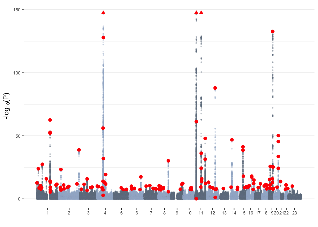 

#dev.off()

# Keep info to summarise in the report below
fastGWA_common=gwas
fastGWA_cojo_common=cojo
fastGWA_clump_common=clump

Red dots represent independent associations identified with COJO.

Summary of results

Briefly, we have:

• 8806780 variants tested – including 260713 in the X chromosome
• 18864 genome-wide significant (GWS; P<5x10^-8) hits – including 527 in the X chromosome
• 143 independent variants (determined with COJO) – including 1 in the X chromosome
• 133 independent variants (determined with COJO) that were GWS in the original GWAS
• 187 independent loci (determined with clumping) – including 1 in the X chromosome
  
  

knownLoci=read.table("input/vitD_knownLoci.txt",h=T,stringsAsFactors=F, sep="\t")
knownLoci=merge(knownLoci, fastGWA_common[,c("SNP","BP")], all.x=T)

# ---------- Check number of new loci in our GWAS - based on COJO results
indep=read.table("results/fastGWA/vitD_fastGWA_withX_conditionOnKnownLoci.gz", h=T, stringsAsFactors=F)
indep_cojo=read.table("results/fastGWA/vitD_fastGWA_withX_conditionOnKnownLoci_maf0.01.cojo", h=T, stringsAsFactors=F)



# ---------- Present table of previously known variants
knownLoci=knownLoci[order(knownLoci$CHR, knownLoci$BP),c("SNP","CHR","BP","ref")]
tmp2=kable(knownLoci, 
           caption=paste0("List of previously reported GWS loci (N=",nrow(knownLoci),")"), 
           row.names=F)
kable_styling(tmp2, full_width=F)

List of previously reported GWS loci (N=6)

SNP	CHR	BP	ref
rs2282679	4	72608383	Ahn et al, Wang et al, Jiang et al
rs10741657	11	14914878	Ahn et al, Wang et al, Jiang et al
rs12785878	11	71167449	Ahn et al, Wang et al, Jiang et al
rs10745742	12	96358529	Jiang et al
rs8018720	14	39556185	Jiang et al
rs6013897	20	52742479	Wang et al, Jiang et al

To assess the number of new associations in our study, we conditioned our results on the list of variants above.

After conditioning on those, we had:

• 14311 GWS associations – including 527 in the X chromosome
• 140 independent variants (determined with COJO) – including 1 in the X chromosome

# ################################################
# Present list of independent associations (identified with COJO)
# ################################################
indep = fastGWA_cojo_common %>% arrange(Chr, bp)

# Format table
indep=indep[,c("Chr","SNP","bp","refA","freq","b","se","p","n","freq_geno","bJ","bJ_se","pJ")]
indep$p=format(indep$p, digits=3)
indep$pJ=format(indep$pJ, digits=3)
indep=indep %>% mutate_at(vars(se, bJ_se, b, bJ), round, 4)
indep=indep %>% mutate_at(vars(freq, freq_geno), round, 2)


# Present table
datatable(indep, 
          rownames=FALSE, 
          extensions=c('Buttons','FixedColumns'),
          options=list(pageLength=5,
                       dom='frtipB',
                       buttons=c('csv', 'excel'),
                       scrollX=TRUE),
          caption="List of independent associations") %>% 
  formatStyle("p","white-space"="nowrap") %>% 
  formatStyle("pJ","white-space"="nowrap")

Columns are: Chr, chromosome; SNP, SNP rs ID; bp, physical position; refA, the effect allele; type, type of QTL; freq, frequency of the effect allele in the original data; b, se and p, effect size, standard error and p-value from the original GWAS; n, estimated effective sample size; freq_geno, frequency of the effect allele in the reference sample; bJ, bJ_se and pJ, effect size, standard error and p-value from a joint analysis of all the selected SNPs.

QQplot + LDSC

To run LDSC, we restricted the GWAS summary statistics to HapMap3 SNPs, excluding the MHC region and X chromosome. For more information see the Methods section above.

# Get sample for QQ plotting
gwas=fastGWA_common
pthrh=0.03
tmp=c(gwas[gwas$P<pthrh,"P"], sample(gwas[gwas$P>pthrh,"P"],100000))

# Plot
qq(tmp)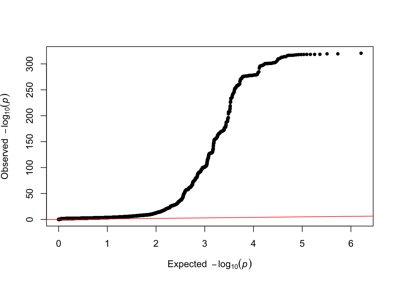

LDSC

tmp=read.table("results/fastGWA/ldsc/vitD_fastGWA.ldsc.log", skip=15, fill=T, h=F, colClasses="character", sep="_")[,1]

# Get results:
h2=strsplit(grep("Total Observed scale h2",tmp, value=T),":")[[1]][2]
lambda_gc=strsplit(grep("Lambda GC",tmp, value=T),":")[[1]][2]
chi2=strsplit(grep("Mean Chi",tmp, value=T),":")[[1]][2]
intercept=strsplit(grep("Intercept",tmp, value=T),":")[[1]][2]
ratio=strsplit(grep("Ratio",tmp, value=T),":")[[1]][2]

• Total Observed scale h²: 0.0966 (0.0138)
• Lambda GC: 1.4817
• Mean Chi²: 1.881
• Intercept: 1.0628 (0.0136)
• Ratio: 0.0713 (0.0154)
  
  

SBayesR

# #########################################
# Run SBayesR
# #########################################

# RCC settings
mldm=$llloyd/sbayesr/pre_review/ukbEURu_hm3_sparse/ukbEURu_hm3_sparse_mldm_list.txt

# Common settings
gctb=$bin/gctb/gctb_2.0_Linux/gctb
prefix=vitD_fastGWA
results=$WD/results/fastGWA
gwas=$results/maFormat/$prefix.ma
output=$results/$prefix.sbayesr

# Run SBayesR
cd $results
tmp_command="$gctb --sbayes R \
                   --gwas-summary $gwas \
                   --mldm $mldm \
                   --out $output"

qsubshcom "$tmp_command" 1 70G $prefix.sbayesr 60:00:00 "$account"


# Copy results to local computer (run command in local computer)
scp $rooID:$WD/results/fastGWA/vitD_fastGWA.sbayesr.parRes $local/results/fastGWA/

tmp=read.table("results/fastGWA/vitD_fastGWA.sbayesr.parRes",h=T,stringsAsFactors=F, skip=2)
h2=round(as.numeric(tmp["hsq",][1]),4)
se=round(as.numeric(tmp["hsq",][2]),4)

• SBayesR h² (SE): 0.1266 (0.0015)