# Libraries 
library(reshape2)
library(ggplot2)
library(knitr)
library(kableExtra)
library(data.table)
library(DT)
library(hrbrthemes)

# Functions
norm = function(x){x[order(x,na.last=NA)]=qnorm(ppoints(length(x[!is.na(x)])),lower=T);x }
se=function(x) {sqrt(var(x,na.rm=TRUE)/length(na.omit(x)))}

# Save results when running all chunks?
saveResults=F
saveplots=F

Variables extracted

To generate phenotype files to use in the GWA analyses, we extracted the following data fields:

f.eid - Individual ID
f.31 - Sex
f.53 - Date of assessment
f.54 - Assessment centre
f.20084 - Vitamin D supplements
f.21001* - BMI
f.21003 - Age when attended assessment centre
f.22000 - Genotype measurement batch
f.30890 - Vitamin D
f.104670 - Vitamin supplement user

Data description

Overview

# Load tidied data
df=read.table("input/vitaminD_tidyData", h=T, stringsAsFactors=F)
df2=reshape2::dcast(df,IID~visit, value.var="vitaminD")

# Sample size with and without vitamin D levels assessed
tot=502536
vitD=nrow(df2)
f=round(vitD/tot*100,2)

# Sample sizes by instance
n1=nrow(df[df$visit=="v0",])
n2=nrow(df[df$visit=="v1",])
n02=nrow(df2[is.na(df2$v0) & !is.na(df2$v1),])
n12=length(unique(df[duplicated(df$IID),"IID"]))

# Restricted to EUR
v3EUR_HM3_IDs=read.table("input/UKB_v3EUR_HM3/ukbEUR_imp_chr1_v3_HM3.fam", h=F, stringsAsFactors=F)
nEUR=nrow(v3EUR_HM3_IDs)
n1_EUR=nrow(df[df$visit=="v0" & df$IID %in% v3EUR_HM3_IDs$V1,])
n02_EUR=nrow(df2[is.na(df2$v0) & !is.na(df2$v1) & df2$IID %in% v3EUR_HM3_IDs$V1,])

# Make table of sample sizes
tmp=data.frame(assessmentTime=c("First assessment at v0","First assessment at v1","Total"),
               All=c(n1, n02, n1+n02),
               Europeans=c(n1_EUR, n02_EUR, n1_EUR+n02_EUR))
names(tmp)[1]=""
tmp=kable(tmp, row.names=F)
kable_styling(tmp, full_width=F)

# Save env
vars2keep=c("f","n02_EUR","n1","n1_EUR","n12","n2","tmp","tot","vitD")
save(list=vars2keep, file = "rdm/input/rmd/dimensions.Rdata")

We have data for 5.02536^{5} individuals. Of those, 449978 (89.54%) have vitamin D levels assessed:

448376 individuals assessed on v0 (2006-2010)
17039 individuals assessed on the v1 (2012-13)

15437 have vitamin D levels measured in both visits.

We restricted our analyses to the 1^st vitamin D measurement that each individual has, and analysed individuals of European ancestry only (N=417580):

	All	Europeans
First assessment at v0	448376	416072
First assessment at v1	1602	1508
Total	449978	417580

Distribution

# Restrict analyses to 1st blood collection only (i.e. remove duplicate observations)
df=read.table("input/vitaminD_tidyData", h=T, stringsAsFactors=F)
df=df[df$analyse=="yes",]
df$analyse=NULL

# Restrict to individuals of European ancestry
df=df[df$IID %in% v3EUR_HM3_IDs$V1,]

# Summary of distribution
#se=function(x) {sqrt(var(x,na.rm=TRUE)/length(na.omit(x)))}

vitD=df$vitaminD
tmp=data.frame(t(unclass(summary(vitD))))
tmp$se=se(vitD); tmp$sd=sd(vitD,na.rm=T)
tmp$N=nrow(df)
tmp2=kable(tmp, caption=paste0("Vitamin D (nmol/L)"), row.names=F)
tmp2=kable_styling(tmp2, full_width=F)

# Density plot of vitamin D
p1=ggplot(df, aes(x=vitaminD)) +
  geom_density(fill="lightcoral", color=alpha("grey", 0),alpha = 0.6) +
  labs(x="25 hydroxyvitamin D (nmol/L)")

# Save env
vars2keep=c("tmp2","p1")
save(list=vars2keep, file = "rdm/input/rmd/distribution.Rdata")

tmp2
p1

Vitamin D (nmol/L)
Min.	X1st.Qu.	Median	Mean	X3rd.Qu.	Max.	se	sd	N
10	33.5	47.9	49.56348	63.2	340	0.0324702	20.9824	417580

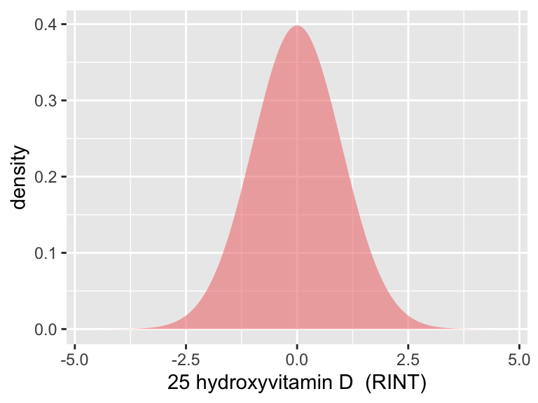
We applied a rank-based inverse-normal transformation to vitamin D levels.

# *************************
# Normalise vitamin D
# *************************
#norm = function(x){x[order(x,na.last=NA)]=qnorm(ppoints(length(x[!is.na(x)])),lower=T);x }
df$norm_vitD=norm(df$vitaminD)
df$log_vitD=log(df$vitaminD)

  ## Save for all descriptive analayses below
  df$season=NULL
  if(saveResults){write.table(df, "input/vitaminD_tidyData_noMissing", quote=F, row.names=F)}

# Summary of normalised distribution
df=read.table("input/vitaminD_tidyData_noMissing", h=T, stringsAsFactors=F)
vitD=df$norm_vitD
tmp=data.frame(t(unclass(summary(vitD))))
tmp$se=se(vitD); tmp$sd=sd(vitD,na.rm=T)
tmp$N=nrow(df)
tmp2=kable(tmp, caption=paste0("Vitamin D (RINT)"), row.names=F)
tmp2=kable_styling(tmp2, full_width=F)

# Density plot of normalised vitamin D
p1=ggplot(df, aes(x=norm_vitD)) +
  geom_density(fill="lightcoral", color=alpha("grey", 0),alpha = 0.6) +
  labs(x="25 hydroxyvitamin D  (RINT)")

# Save env
vars2keep=c("tmp2","p1")
save(list=vars2keep, file = "rdm/input/rmd/nomalised_distribution.Rdata")

tmp2
p1

Vitamin D (RINT)
Min.	X1st.Qu.	Median	Mean	X3rd.Qu.	Max.	se	sd	N
-4.716892	-0.6744879	0	0	0.6744879	4.716892	0.0015475	0.9999996	417580

Time series

Vitamin D in Year-Months

df=read.table("input/vitaminD_tidyData_noMissing", h=T, stringsAsFactors=F)

# *************************
# Average
# *************************
# Calculate average and 95% CI in each month
df$assessMonthYear=substr(df$assessDate,1,7)
df_YMmeans = do.call(data.frame,aggregate(norm_vitD ~ assessMonthYear+visit, df, function(x)c(mean=mean(x), sd=sd(x), N=length(x))))
names(df_YMmeans)[3:5] = c("norm_vitD","sd","N")
df_YMmeans$minCI = df_YMmeans$norm_vitD - 1.96*df_YMmeans$sd/sqrt(df_YMmeans$N)
df_YMmeans$maxCI = df_YMmeans$norm_vitD + 1.96*df_YMmeans$sd/sqrt(df_YMmeans$N)

# Sample size per month
tmp=data.frame(table(df$assessMonthYear, df$visit))
tmp=tmp[tmp$Freq!=0,]
names(tmp)=c("ym","visit","freq")

# Remove outliers
outliers=head(tmp[order(tmp$freq),])
df_YMmeans=df_YMmeans[!df_YMmeans$assessMonthYear %in% outliers[outliers$freq<30,"ym"],]

# Change visit labels
df_YMmeans$visit=factor(df_YMmeans$visit, labels=c("Baseline", "Follow-up"))

# Plot monthly average
p1=ggplot(df_YMmeans, aes(x=assessMonthYear, y=norm_vitD, group=visit)) +
  geom_ribbon(aes(ymin=minCI,ymax=maxCI),alpha=0.3, color=NA, fill="lightcoral")+
  geom_line(size=1.1, col="lightcoral") +
  geom_point(size=4, aes(shape=visit), fill="white", col="lightcoral") +
  scale_shape_manual(values = c(22, 24)) +
  theme(text = element_text(size=13),
        axis.text.x = element_text(angle = 45, vjust = 1, hjust=1),
        legend.title = element_blank(),
        legend.position = "none",
        plot.background = element_rect(fill="transparent",colour = NA)) +
  labs(y="Average 25 hydroxyvitamin D\n(RINT)", x=paste0("Month and Year of assessment")) +
  theme(plot.caption = element_text(hjust = 0))

# Save env
vars2keep=c("tmp","p1")
save(list=vars2keep, file = "rdm/input/rmd/vitD_ym.RData")

if(saveplots){tiff("manuscript/Figures/figureS1_25OHD_mean_RINT_YM.tiff", width=10, height=4 ,units="in", res=800,compression = "lzw", bg="transparent")}
p1
if(saveplots){dev.off()}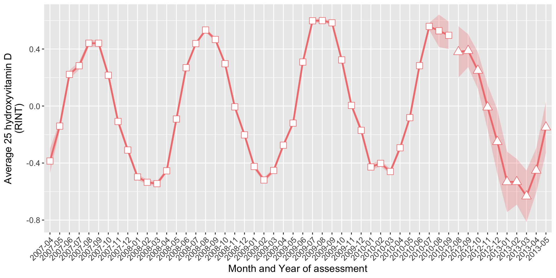

On average:

9456 individuals were assessed per month in the first visit (v0)
137 individuals were assessed per month in the repeat visit (v1)

Vitamin D in each month (all years aggregated)

df=read.table("input/vitaminD_tidyData_noMissing", h=T, stringsAsFactors=F)

# *************************
# Average
# *************************
# ----- Monthly mean of 25OHD (obs scale)

  # Calculate average and 95% CI in each month
  tmp = do.call(data.frame,aggregate(vitaminD ~ assessMonth, df, function(x)c(mean=mean(x), sd=sd(x), N=length(x))))
  names(tmp)[2:4] = c("vitD","sd","N")
  tmp[tmp$assessMonth>=12 | tmp$assessMonth<=4,"season"]="winter"
  tmp[tmp$assessMonth>=6 & tmp$assessMonth<=10,"season"]="summer"
  tmp[tmp$assessMonth==5 | tmp$assessMonth==11,"season"]="N/A"
  tmp$season=factor(tmp$season, levels=c("summer","winter","N/A"))
  tmp$minCI = tmp$vitD - 1.96*tmp$sd/sqrt(tmp$N)
  tmp$maxCI = tmp$vitD + 1.96*tmp$sd/sqrt(tmp$N)

  # Plot
  p1=ggplot(data=tmp, aes(x=assessMonth, y=vitD, group=1)) +
    geom_ribbon(data=tmp,aes(ymin=minCI,ymax=maxCI), alpha=0.4, color=NA, fill="grey") +
    geom_line(size=1, col="grey") +
    geom_point(size=5, aes(col=season)) +
    scale_color_manual(values=c("orange","cadetblue","grey")) +
    theme(legend.title = element_blank(),
          legend.position = "none",
          plot.background = element_rect(fill="transparent",colour = NA)) +
    scale_x_continuous(breaks=seq(1,12,1)) +
    labs(y="Average 25 hydroxyvitamin D (nmol/L)", x=paste0("Month of assessment")) 
  
  if(saveplots){tiff("manuscript/Figures/figureS1_25OHD_mean_obsScale.tiff", width=5, height=4 ,units="in", res=800,compression = "lzw", bg="transparent")}
  p1
  if(saveplots){dev.off()}

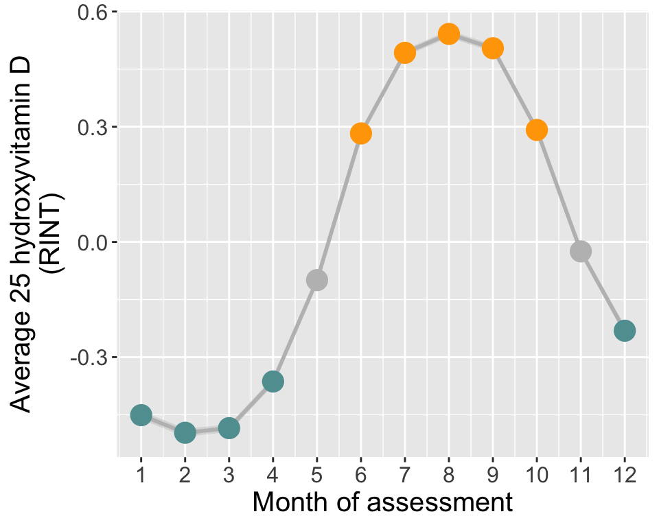
# ----- Monthly mean of 25OHD (RINT)

  # Calculate average and 95% CI in each month
  tmp = do.call(data.frame,aggregate(norm_vitD ~ assessMonth, df, function(x)c(mean=mean(x), sd=sd(x), N=length(x))))
  names(tmp)[2:4] = c("vitD","sd","N")
  tmp[tmp$assessMonth>=12 | tmp$assessMonth<=4,"season"]="winter"
  tmp[tmp$assessMonth>=6 & tmp$assessMonth<=10,"season"]="summer"
  tmp[tmp$assessMonth==5 | tmp$assessMonth==11,"season"]="N/A"
  tmp$season=factor(tmp$season, levels=c("summer","winter","N/A"))
  tmp$minCI = tmp$vitD - 1.96*tmp$sd/sqrt(tmp$N)
  tmp$maxCI = tmp$vitD + 1.96*tmp$sd/sqrt(tmp$N)

  # Plot
  p2=ggplot(data=tmp, aes(x=assessMonth, y=vitD, group=1)) +
    geom_ribbon(data=tmp,aes(ymin=minCI,ymax=maxCI), alpha=0.4, color=NA, fill="grey") +
    geom_line(size=1, col="grey") +
    geom_point(size=5, aes(col=season)) +
    scale_color_manual(values=c("orange","cadetblue","grey")) +
    theme(text = element_text(size=15),
          legend.title = element_blank(),
          legend.position = "none",
          plot.background = element_rect(fill="transparent",colour = NA)) +
    scale_x_continuous(breaks=seq(1,12,1)) +
    labs(y="Average 25 hydroxyvitamin D\n(RINT)", x=paste0("Month of assessment")) 
  
  if(saveplots){tiff("manuscript/Figures/figureS1_25OHD_mean_RINT.tiff", width=5, height=4 ,units="in", res=800,compression = "lzw", bg="transparent")}
  p2
  if(saveplots){dev.off()}



# *************************
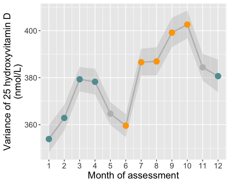
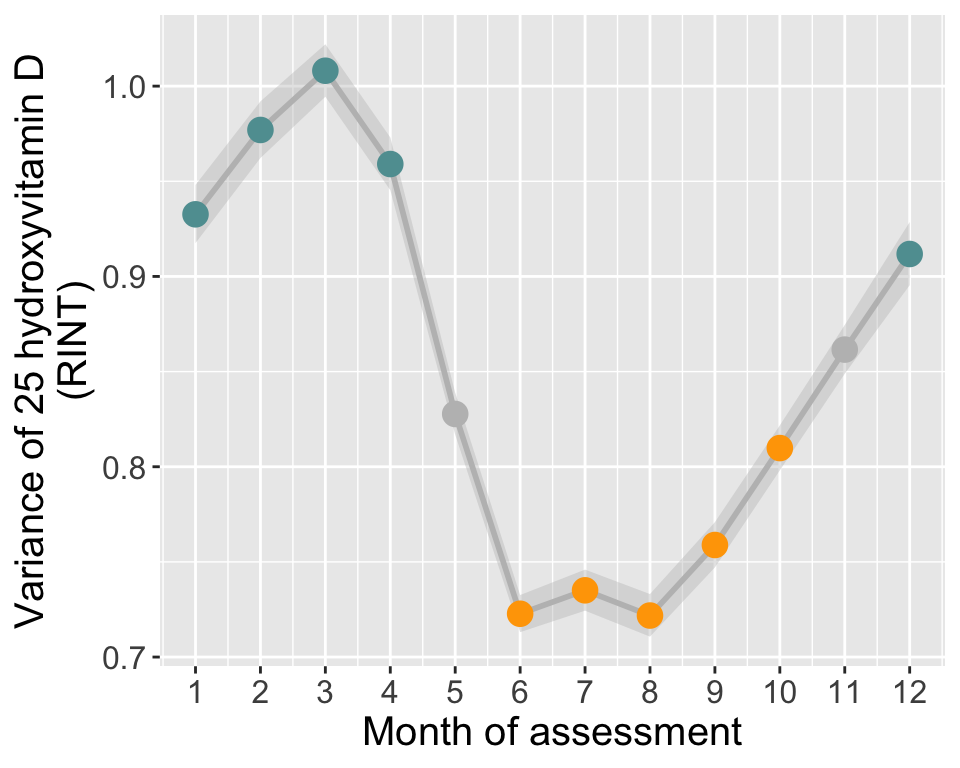
# Variance
# *************************
 # Calculate variance and 95% CI in each month
  tmp = do.call(data.frame,aggregate(vitaminD ~ assessMonth, df, function(x)c(var=var(x), N=length(x))))
  names(tmp)[2:3] = c("vitD_s2","N")
  tmp[tmp$assessMonth>=12 | tmp$assessMonth<=4,"season"]="winter"
  tmp[tmp$assessMonth>=6 & tmp$assessMonth<=10,"season"]="summer"
  tmp[tmp$assessMonth==5 | tmp$assessMonth==11,"season"]="N/A"
  tmp$season=factor(tmp$season, levels=c("summer","winter","N/A"))
  chi2_0.025=qchisq(0.025,tmp$N)
  chi2_0.975=qchisq(0.975,tmp$N)
  tmp$minCI = (tmp$N-1)*tmp$vitD_s2/chi2_0.975
  tmp$maxCI = (tmp$N-1)*tmp$vitD_s2/chi2_0.025

  # Plot
  p3=ggplot(data=tmp, aes(x=assessMonth, y=vitD_s2, group=1)) +
    geom_ribbon(data=tmp,aes(ymin=minCI,ymax=maxCI),alpha=0.4, color=NA, fill="grey")+
    geom_line(size=1, color="grey") +
    geom_point(size=4, aes(col=season)) +
    scale_color_manual(values=c("orange","cadetblue","grey")) +
    scale_shape_manual(values = c(21, 24)) +
    theme(text = element_text(size=15),
          legend.title = element_blank(),
          legend.position = "none",
          plot.background = element_rect(fill="transparent",colour = NA)) +
    scale_x_continuous(breaks=seq(1,12,1)) +
    labs(y="Variance of 25 hydroxyvitamin D\n(nmol/L)", x=paste0("Month of assessment")) 

  if(saveplots){tiff("manuscript/Figures/figureS1_25OHD_variance_obsScale.tiff", width=5, height=4 ,units="in", res=800,compression = "lzw", bg="transparent")}
  p3
  if(saveplots){dev.off()}

# ----- Monthly variance of 25OHD (RINT)

  # Calculate variance and 95% CI in each month
  tmp = do.call(data.frame,aggregate(norm_vitD ~ assessMonth, df, function(x)c(var=var(x), N=length(x))))
  names(tmp)[2:3] = c("vitD_s2","N")
  tmp[tmp$assessMonth>=12 | tmp$assessMonth<=4,"season"]="winter"
  tmp[tmp$assessMonth>=6 & tmp$assessMonth<=10,"season"]="summer"
  tmp[tmp$assessMonth==5 | tmp$assessMonth==11,"season"]="N/A"
  tmp$season=factor(tmp$season, levels=c("summer","winter","N/A"))
  chi2_0.025=qchisq(0.025,tmp$N)
  chi2_0.975=qchisq(0.975,tmp$N)
  tmp$minCI = (tmp$N-1)*tmp$vitD_s2/chi2_0.975
  tmp$maxCI = (tmp$N-1)*tmp$vitD_s2/chi2_0.025

  # Plot
  p4=ggplot(data=tmp, aes(x=assessMonth, y=vitD_s2, group=1)) +
    geom_ribbon(data=tmp,aes(ymin=minCI,ymax=maxCI),alpha=0.4, color=NA, fill="grey")+
    geom_line(size=1, color="grey") +
    geom_point(size=4, aes(col=season)) +
    scale_color_manual(values=c("orange","cadetblue","grey")) +
    scale_shape_manual(values = c(21, 24)) +
    theme(text = element_text(size=15),
          legend.title = element_blank(),
          legend.position = "none",
          plot.background = element_rect(fill="transparent",colour = NA)) +
    scale_x_continuous(breaks=seq(1,12,1)) +
    labs(y="Variance of 25 hydroxyvitamin D\n(RINT)", x=paste0("Month of assessment")) 
  
  if(saveplots){tiff("manuscript/Figures/figureS1_25OHD_variance_RINT.tiff", width=5, height=4 ,units="in", res=800,compression = "lzw", bg="transparent")}
  p4
  if(saveplots){dev.off()}

# Save env
vars2keep=c("p1","p2","p3","p4")
save(list=vars2keep, file = "rdm/input/rmd/vitD_monthly_mean_and_var.RData")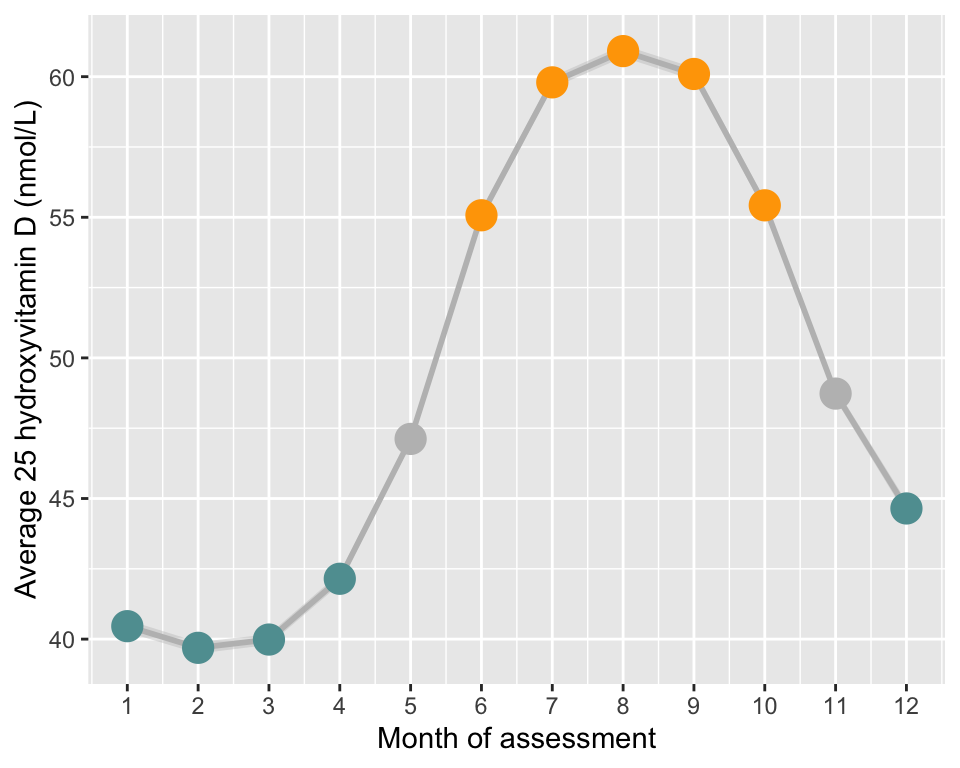

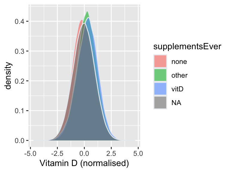
Vitamin D supplements

Field 104670 indicates whether individuals replied to the survey on supplement intake.

For individuals who replied yes, field 20084 summaries which supplements they took. Individuals with code 479 in that question indicated that they had vitamin D supplements the day before the questionnaire.

Fields 104670 and 20084 were assessed at 5 instances:

instance 0: April 2009 to September 2010
instance 1: February 2011 to April 2011
instance 2: June 2011 to September 2011
instance 3: October 2011 to December 2011
instance 4: April 2012 to June 2012

Vitamin D in individuals with/without supplements at any time point

Using information from all time-points, the following groups were defined:

NA: Individuals with no information on supplements taken (ever)
none: Individuals who always reported not taking supplements
other: Individuals who always reported taking other supplements (not vitamin D)
vitD: Individuals who ever reported taking vitamin D (may also have taken other supplements)

As before, the group no-vitD was obtained by grouping individuals in the categories none and other.

df=read.table("input/vitaminD_tidyData_noMissing", h=T, stringsAsFactors=F)

# Summary in individuals with no supplement information
vitD=df[is.na(df$supplementsEver),"norm_vitD"]
n=length(vitD)
tmp=data.frame(t(unclass(summary(vitD))))
tmp$se=se(vitD); tmp$sd=sd(vitD,na.rm=T); tmp$N=n
tmp$supplementGroup="NA"
df2=tmp[,c(ncol(tmp), ncol(tmp)-1,1:(ncol(tmp)-2))]

# Summary in individuals with supplement information
for(i in c("none","other","vitD"))
{
  vitD=df[!is.na(df$supplementsEver) & df$supplementsEver==i,"norm_vitD"]
  n=length(vitD)
  tmp=data.frame(t(unclass(summary(vitD))))
  tmp$se=se(vitD); tmp$sd=sd(vitD,na.rm=T); tmp$N=n 
  tmp$supplementGroup=i
  df2=rbind(df2, tmp[,names(df2)])
}

# Summary in individuals with no vitD supplements (i.e. 'none'+'other')
vitD=df[!is.na(df$supplementsEver) & df$supplementsEver %in% c("none","other"),"norm_vitD"]
n=length(vitD)
tmp=data.frame(t(unclass(summary(vitD))))
tmp$se=se(vitD); tmp$sd=sd(vitD,na.rm=T); tmp$N=n
tmp$supplementGroup="no-vitD"
df2=rbind(df2, tmp[,names(df2)])

# Summary in individuals with ever vitamin D vs. never/NA
df$supplementGroup=ifelse(!is.na(df$supplements) & df$supplements=="vitD", "ever", "never/NA")
vitD=df[df$supplementGroup=="never/NA","norm_vitD"]
n=length(vitD)
tmp=data.frame(t(unclass(summary(vitD))))
tmp$se=se(vitD); tmp$sd=sd(vitD,na.rm=T); tmp$N=n
tmp$supplementGroup="never/NA (none+other+NA)"
df2=rbind(df2, tmp[,names(df2)])


# Summary table for all groups above
tmp2=kable(df2, caption=paste0("Vitamin D (normalised) by supplement group - EVER"), row.names=F)
tmp2=kable_styling(tmp2, full_width=F)


# Density plot by supplement group
p1=ggplot(df, aes(x=norm_vitD)) +
  geom_density(aes(fill=supplementsEver), color="#e9ecef",alpha = 0.6) +
  xlab("Vitamin D (normalised)")

# Density plot by supplement group: ever vs. never/NA
p2=ggplot(df, aes(x=norm_vitD)) +
  geom_density(aes(fill=supplementGroup), color="#e9ecef",alpha = 0.6) +
  xlab("Vitamin D (normalised)")

# Save env
vars2keep=c("p1","p2","tmp2")
save(list=vars2keep, file = "rdm/input/rmd/dist_by_supp.RData")

Vitamin D (normalised) by supplement group - EVER
supplementGroup	N	Min.	X1st.Qu.	Median	Mean	X3rd.Qu.	Max.	se	sd
NA	238090	-4.716892	-0.7236918	-0.0414398	-0.0407201	0.6418865	4.378065	0.0020718	1.0109343
none	90992	-4.304144	-0.7914820	-0.1441555	-0.1211890	0.5305524	4.716892	0.0032528	0.9812146
other	76863	-3.947332	-0.3846385	0.2374143	0.2283545	0.8575268	4.248166	0.0034084	0.9449495
vitD	11635	-3.733036	-0.3782312	0.3038705	0.2724769	0.9492897	4.132261	0.0091830	0.9905259
no-vitD	167855	-4.304144	-0.6208657	0.0357630	0.0388716	0.6970480	4.716892	0.0023929	0.9803668
never/NA (none+other+NA)	415693	-4.716892	-0.6772090	-0.0031484	-0.0029033	0.6712566	4.716892	0.0015505	0.9996895

In the plot below, the following groups were used:

ever: vitamin D reported at any of the 5 time points (may also have taken other supplements). Equivalent to vitD above.
never/NA: individuals who (1) never reported taking vitamin D (may have reported other supplements or not taking supplements ever) or (2) never replied to the supplement questionnaire. This is equivalent to other+none+NA.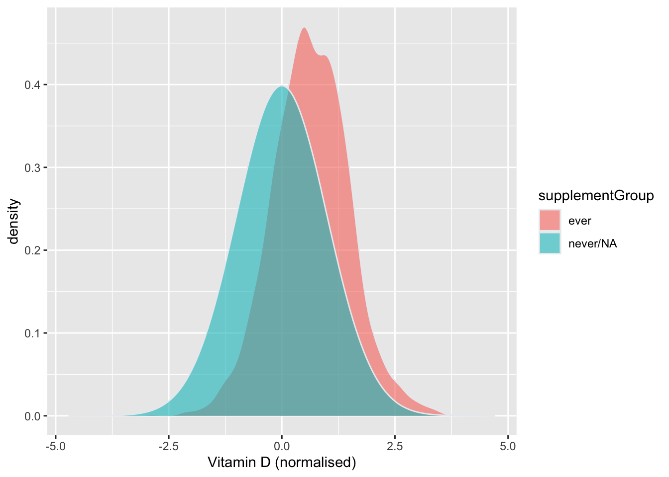

Covariates

Principal components

We included principal components (PCs) in our GWAS to account for population stratification. Specifically, we used 40 PCs generated with FlashPCA, using ~500K HapMap3 SNPs and excluding regions of long-range LD (LD<0.9).

Association tests with covariates

In this section we tested the association between potential confounder variables and normalised vitamin D levels.

df=read.table("input/vitaminD_tidyData_noMissing", h=T, stringsAsFactors=F)
df$assessMonthYear=substr(df$assessDate,1,7)
load("input/ukbEUR_PC40_HM3excludeRegions_v2.RData")

# Create file with phenotype and covariates to analyse
df2=df[,c("IID","vitaminD","norm_vitD","log_vitD","sex","age","bmi","batch","assessCentre","assessMonth","assessMonthYear","supplementsEver")]
df2=merge(df2, pcs[,2:12], all.x=T)
  catVars=c("assessCentre","assessMonth","assessMonthYear","batch","supplementsEver")
  df2[,catVars] = lapply(df2[,catVars], factor)

# Create a table to keep results from all association tests
out=data.frame(covariate=names(df2)[-c(1:4)],
               test="lm",beta=NA, r2=NA, p=NA, stringsAsFactors=F)
out[out$covariate %in% catVars,"test"]="anova"
out2=c()
for(iv in c("vitaminD","norm_vitD","log_vitD"))
{
  tmp=out
  tmp$IV=iv
  out2=rbind(out2,tmp)
}
out=out2

# Run associations
for (i in 1:nrow(out))
{
  iv=out[i,"IV"]
  c=out[i,"covariate"]
  
  if(!c %in% catVars)
  {
    model=lm(df2[,iv]~df2[,c])
    r2=summary(model)$r.squared
    coef=summary(model)$coefficients
    beta=round(coef[2,1],3)
    p=coef[2,4]
  }
  
  if(c %in% catVars)
  {
    model=lm(df2[,iv]~df2[,c])
    r2=summary(model)$r.squared
    coef=summary(aov(df2[,iv]~df2[,c]))
    beta=NA
    p=coef[[1]][["Pr(>F)"]][1]
  }
  
  out[i,c("beta","r2","p")]=c(beta, 
                              format(r2, digits=2), 
                              format(p, digits=3))
}

# Run a few extra associations
if(F)
{
  df2=merge(df2, pcs[,c(2,13:42)], all.x=T)
  lmp <- function (modelobject) {
    if (class(modelobject) != "lm") stop("Not an object of class 'lm' ")
    f <- summary(modelobject)$fstatistic
    p <- pf(f[1],f[2],f[3],lower.tail=F)
    attributes(p) <- NULL
    return(p)}
  tmp=c()
  # All 40 PCs
  for(iv in c("vitaminD","norm_vitD","log_vitD"))
  {
    fixed=paste(paste0("PC",1:40), collapse="+")
    model = as.formula(paste("df[,",iv,"]~",fixed))
    test=lm(model, data=df2)      
    r2=summary(test)$r.squared
  p=lmp(test)
  tmp=data.frame(covariate="First 40 PCs", test="lm", beta=NA, r2=r2, p=p, IV=iv)
  }
  

}

# Show results
out$p=format(out$p, digits=3)
out$p=as.character(out$p)
out=dcast(setDT(out), covariate +test ~ IV, value.var=c("beta","r2","p"))

# Save env
save(out, file = "rdm/input/rmd/cov_associations.RData")

datatable(out, 
        rownames=FALSE, 
        extensions=c('Buttons','FixedColumns'),
        options=list(dom='frtipB',
                     buttons=c('csv', 'excel'),
                     scrollX=TRUE),
        caption="Covariate association results with vitamin D (raw, RINT, and log-transformed)")

Prepare file with covariates to include in MLM GWAS

We fit the following variables in the mixed linear model (MLM) analyses:

Age
Sex
Assessment month
Assessment centre
First 40 PCs
Genotyping batch
Supplement intake: As defined above.

df=read.table("input/vitaminD_tidyData_noMissing", h=T, stringsAsFactors=F)
#load("input/ukbEUR_PC40_HM3excludeRegions_v2.RData")

# ---- Categorical confounders
df$FID=df$IID
catCov=df[,c("FID","IID","sex","batch","assessCentre","assessMonth","supplementsEver")]
catCov[is.na(catCov$supplementsEver),"supplementsEver"]="NoInfo"

  # Create file with no sex for X chromosome analyses (which are run individually in males and females)
  catCov_noSex=catCov[,grep("sex",names(catCov), invert=T)]

# ---- Quantitative confounders
quantCov=df[,c("FID","IID","age")]
quantCov=merge(quantCov, pcs[,2:42], all.x=T)
names(quantCov)[1:2]=c("FID","IID")

  # Create a file with BMI as well
  quantCov_bmi=df[,c("FID","IID","age","bmi")]
  quantCov_bmi=merge(quantCov_bmi, pcs[,2:42], all.x=T)
  names(quantCov_bmi)[1:2]=c("FID","IID")


# ---- Save files 
if(saveResults){write.table(catCov, "input/categoricalCovariates", quote=F, row.names=F)}
if(saveResults){write.table(catCov_noSex, "input/categoricalCovariates_noSex", quote=F, row.names=F)}
if(saveResults){write.table(quantCov, "input/quantitativeCovariates", quote=F, row.names=F)}
if(saveResults){write.table(quantCov_bmi, "input/quantitativeCovariates_bmi", quote=F, row.names=F)}

Prepare phenotype

In this section, we prepared the phenotypes for the following analyses:

fastGWA

The main GWA analyses were conducted with the mixed linear model (MLM) implemented in fastGWA

To generate the phenotype for those analyses, we:

Restricted our sample to the full set of individuals with European ancestry
Normalised phenotype with a rank-based inverse normal transformation (RINT)

Covariates were included in the GWA model to correct for confounder effects. The list of confouders used is in the Covariate section

# Restrict to ALL individuals of European ancestry
v3EUR_HM3_IDs=read.table("input/UKB_v3EUR_HM3/ukbEUR_imp_chr1_v3_HM3.fam", h=F, stringsAsFactors=F)
names(v3EUR_HM3_IDs)[1:2]=c("FID","IID")
df=read.table("input/vitaminD_tidyData_noMissing", h=T, stringsAsFactors=F)
df2=df[df$IID %in% v3EUR_HM3_IDs$IID,]

# Save log-transformed and RINT phenotype (to assess validity of meta-analysis)
if(saveResults){write.table(df2[,c("IID","log_vitD","norm_vitD")], "tmpDir/mlm_norm_log_pheno", row.names=F, quote=F)}

# Save normalised residuals to feed as phenotype to the fastGWA and BOLT-LMM
df2=df2[,c("IID","norm_vitD")]
df2$FID=df2$IID
df2=df2[,c("FID","IID","norm_vitD")]
if(saveResults){write.table(df2, "input/mlm_pheno", row.names=F, quote=F)}

Meta-analysis

To meta-analyse UKB results with results obtained by the SUNLIGHT consortium, we analysed the data in the same way, i.e.:

Restricting data to individuals of European ancestry
Using a log-transformed phenotype
Including the following covariates in the model (fastGWA):
- Assessment month
- Age
- Sex
- BMI
- 40 PCs
- Genotyping batch

# Code from Jenny

Season-stratified GWAS

# Restrict to ALL individuals of European ancestry
df=read.table("input/vitaminD_tidyData_noMissing", h=T, stringsAsFactors=F)
df2=df
df2$FID=df2$IID

# Define seasons
## Winter = Dec - Apr
## Summer = Jun - Oct
df2$season=NULL
df2[df2$assessMonth<=4 | df2$assessMonth>=12,"season"]="winter"
df2[df2$assessMonth>=6  & df2$assessMonth<=10,"season"]="summer"
df2=df2[!is.na(df2$season),]

# stratify data and apply RINT
  # Summarise
  winter=df2[df2$season=="winter",c("FID","IID","vitaminD","norm_vitD","log_vitD")]
  summer=df2[df2$season=="summer",c("FID","IID","vitaminD","norm_vitD","log_vitD")]
  summary(summer$vitaminD); sd(summer$vitaminD); summary(winter$vitaminD); sd(winter$vitaminD)
  #summary(summer$norm_vitD); sd(summer$norm_vitD); summary(winter$norm_vitD); sd(winter$norm_vitD)
  #summary(summer$log_vitD); sd(summer$log_vitD); summary(winter$log_vitD); sd(winter$log_vitD)
winter=df2[df2$season=="winter",c("FID","IID","norm_vitD")]
summer=df2[df2$season=="summer",c("FID","IID","norm_vitD")]
norm = function(x){x[order(x,na.last=NA)]=qnorm(ppoints(length(x[!is.na(x)])),lower=T);x }
winter$norm_vitD=norm(winter$norm_vitD)
summer$norm_vitD=norm(summer$norm_vitD)

# Save "season" definition
df2$season_binary=ifelse(df2$season=="winter", 1, 2)
df2=df2[,c("FID","IID","norm_vitD","season","season_binary")]
if(saveResults){write.table(df2, "input/covariates_season", row.names=F, quote=F)}

# Save datasets to feed as phenotype to fastGWA
if(saveResults){write.table(winter, "input/mlm_winter_pheno", row.names=F, quote=F)}
if(saveResults){write.table(summer, "input/mlm_summer_pheno", row.names=F, quote=F)}

After a visual inspection of the average vitamin D levels per month (see Time series section), we defined two seasons of blood draw and stratified the UKB sample into two cohorts based on those:

“Winter” - individuals assessed Dec-Apr (N=162591)
“Summer” - individuals assessed Jun-Oct (N=177082)

Individuals with vitamin D levels assessed in the months of May and November were not included in these analyses as the transition between seasons varies between years and could confound the results.

The two phenotype files (one for each season) were generated by (1) restricting to individuals of European ancestry, (2) restricting the individuals assessed in the defined season and (3) applying a rank-based inverse-normal transformation.

vQTL GWAS

The phenotype used in the variance quantitative trait loci (vQTL) GWAS was pre-regressed of confounder effects. Briefly, we:

Restricted to unrelated European individuals
Regressed-out the effect of confounders within the following groups:
- Females-vitD: females who ever reported taking vitamin D supplements (vitD group)
- Females-other: females who ever reported taking supplements, but never vitamin D (other group)
- Females-none: females who always reported not taking supplements (none group)
- Females-NA females with no information on supplement intake (NA group)
- Males-vitD: males who ever reported taking vitamin D supplements (vitD group)
- Males-other: males who ever reported taking supplements, but never vitamin D other group)
- Males-none: males who always reported not taking supplements (none group)
- Males-NA: males with no information on supplement intake NA group)
Removed outliers more than 5 SD from the mean
Standardised the residuals to get mean 0 and SD 1 (note that this is not a non-linear transformation and will help with interpretation of downstream analyses)
Merged residuals from the different groups

Variables regressed from the phenotype were:

Age
Assessment month
Assessment centre
First 40 PCs
Genotyping batch

# Add PCs to our data frame to remove their effect
df=read.table("input/vitaminD_tidyData_noMissing", h=T, stringsAsFactors=F)
#load("input/ukbEUR_PC40_HM3excludeRegions_v2.RData")
df2=merge(df, pcs, all.x=T)

# Restrict to unrelated individuals of European ancestry
v3EURu_HM3_IDs=read.table("input/ukbEURu_imp_chr1_v3_HM3.fam", h=F, stringsAsFactors=F)
#nrow(v3EURu_HM3_IDs)
names(v3EURu_HM3_IDs)[1:2]=c("FID","IID")
df2=df2[df2$IID %in% v3EURu_HM3_IDs$IID,]
#length(df2$IID)

There were 348,501 unrelated individuals of European ancestry. Of those, 318,851 had vitamin D levels assessed and will be analysed in this preliminary analysis.

# Show sample size of the groups within which we will run covariate regression
tmp=table(df2$sex, df2$supplementsEver, exclude=NULL)
tmp=kable(tmp, caption="Sample size of groups within which we ran covariate regression")
t1=kable_styling(tmp, full_width=F)

# Define the groups within which we will run covariate regression
df2[is.na(df2$supplementsEver),"supplementsEver"]="NA"
df2$group=paste(df2$sex, df2$supplementsEver, sep="_")

# Code categorical variables as factors
df2[,c("assessCentre","assessMonth","batch")] = lapply(df2[,c("assessCentre","assessMonth","batch")], factor)

# Regress effect of covariates
nPCs=40 # number of PCs to include
for(i in unique(df2$group))
{
  # Get residuals
  test=paste("vitaminD ~ age + assessCentre + assessMonth + batch +", paste(paste0("PC",1:nPCs),collapse = "+"))
  model=lm(as.formula(test), df2[df2$group==i,])
  res=resid(model)
  
  # Remove outliers (>5 SD from mean)
  low=mean(res)-5*sd(res)
  high=mean(res)+5*sd(res)
  res[res<low | res>high]=NA
  
  # Standardize residuals for mean 0 and SD 1 (note: this is not a non-lienar transformation and will help with the interpretation of the results)
  res_std=(res-mean(res, na.rm=T))/sd(res, na.rm=T)
  
  # Add standardized residuals to data frame
  df2[df2$group==i,"vitD_res"]=res_std
}
df2=df2[!is.na(df2$vitD_res),]



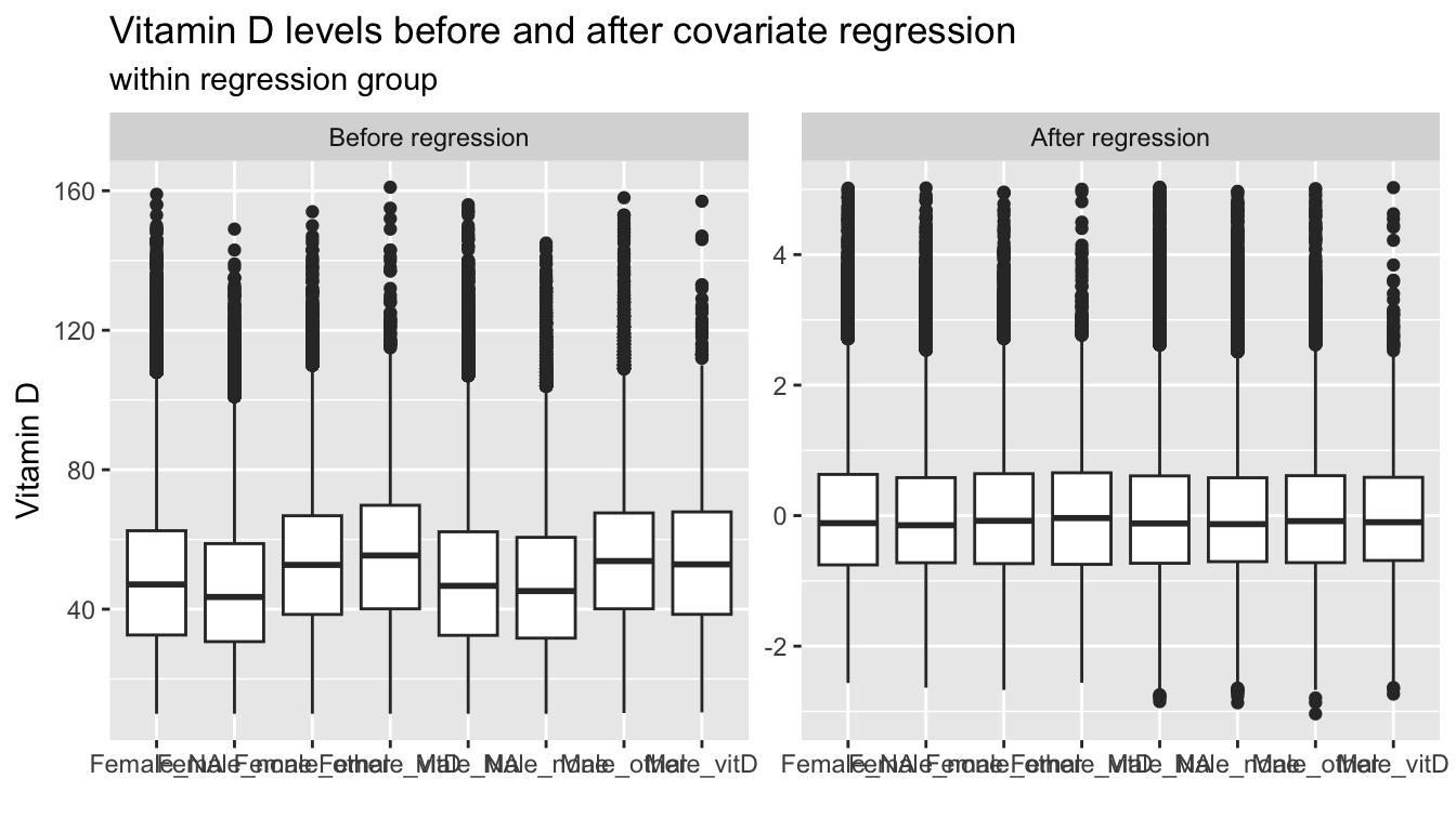
# Plot residuals by group
tmp=reshape2::melt(df2[,c("IID","vitaminD","vitD_res","group")], id.vars=c("IID", "group"))
tmp$variable=factor(tmp$variable, levels=c("vitaminD","vitD_res"), labels=c("Before regression","After regression"))
p1=ggplot(tmp, aes(x=group, y=value)) +
  geom_boxplot() +
  facet_wrap(variable~., scales="free") +
  labs(title="Vitamin D levels before and after covariate regression",
       subtitle="within regression group",
       x="",y="Vitamin D")

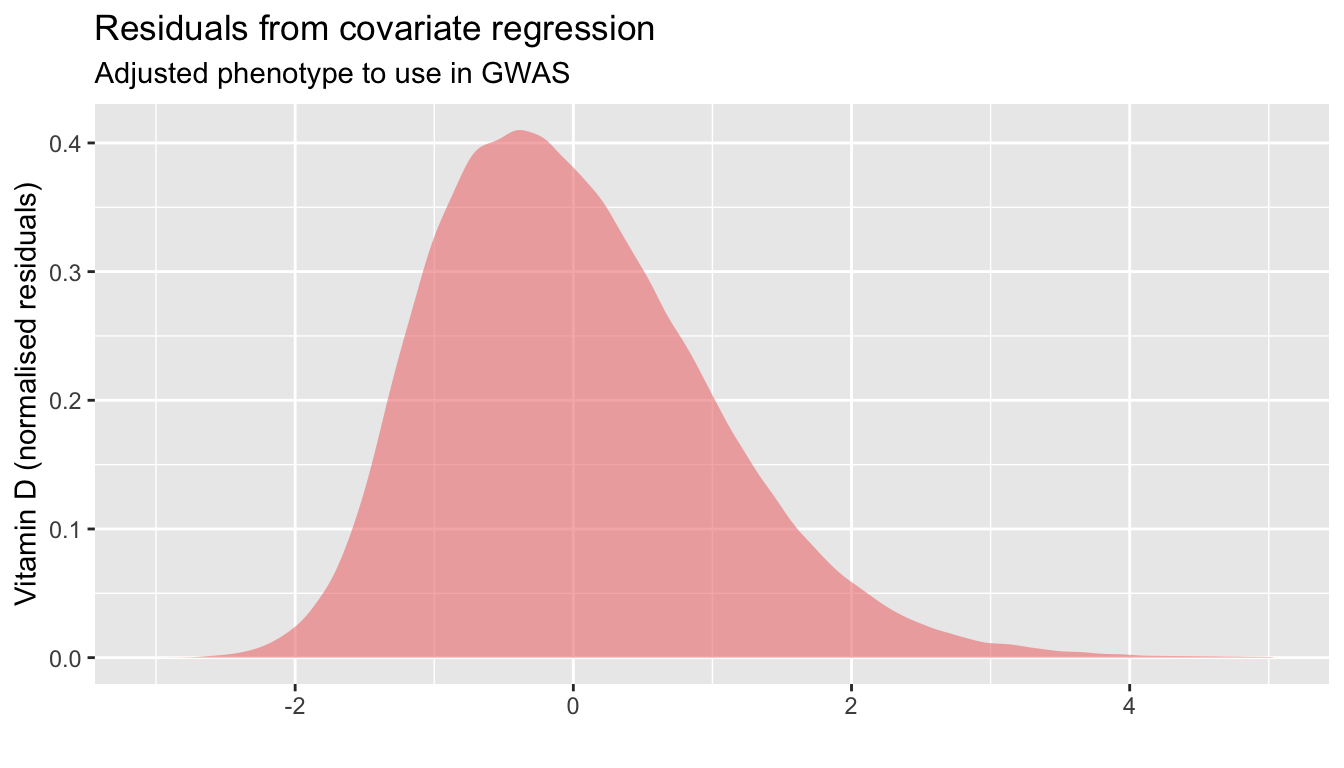
# Plot adjusted phenotype
p2=ggplot(df2, aes(x=vitD_res)) +
  geom_density(fill="lightcoral", color=alpha("grey", 0),alpha = 0.6) +
  labs(title="Residuals from covariate regression",
       subtitle="Adjusted phenotype to use in GWAS",
       x="",y="Vitamin D (normalised residuals)")

# Save  residuals to feed as phenotype for the vQTL GWAS
df2=df2[,c("IID","vitD_res")]
df2$FID=df2$IID
df2=df2[,c("FID","IID","vitD_res")]
if(saveResults){write.table(df2, "input/vqtl_pheno", row.names=F, quote=F)}

# Save env
vars2keep=c("p1","p2","t1")
save(list=vars2keep, file = "rdm/input/rmd/vqtl_cov_regression.RData")

t1;p1;p2

Sample size of groups within which we ran covariate regression
	none	other	vitD	NA
Female	34278	35309	6624	93901
Male	36969	24897	2655	84218

25OHD phenotype